Summary
Nearly 50 new functions have been added to Excel! This is not your Dad's Excel anymore – a lot has changed. This article takes a quick tour of the new functions, with links to more detailed information.
For a very long time, Excel introduced new functions at a leisurely pace. Every few years, a handful of new functions would appear, most aimed at technical and edge-case problems. Most users greeted these new functions with a yawn, if they noticed at all.
All that changed in 2019 when Microsoft's Excel team kicked things into high gear and suddenly began introducing brand-new functions at a furious pace. You might not know it, but Excel now has nearly 50 new functions! At the same time, Microsoft overhauled Excel's formula engine to handle array formulas natively. The name "array formulas" may seem dreadfully dull (for super-geeks only), but this upgrade affects literally everything in Excel (even basic worksheets) because Excel can now return multiple results. Need a list of unique values from 10,000 rows? The UNIQUE function will do it in one step. Want to display all orders over $100? Done! With the new FILTER function. Even better, because these are formulas, the results are dynamic. When data changes, you see the latest immediately.
This is not your Dad's Excel anymore. The new upgraded engine and new functions are a massive change that will ripple through business and personal spreadsheets for years to come. Many complicated formulas will become obsolete, replaced by compact and elegant alternatives. If you use Excel frequently, this is a change you should understand and embrace. To help you get started, below is a list of new functions since Excel 2019, when everything began to change. Use the links to see more details and examples.
Table of contents
Excel versions
As Excel 365 has become more widely used, understanding Excel versions has become more complicated. Here's how it works.
- New functions are first introduced to the "Beta" channel for Excel 365. This is a special channel that you must opt in to specifically. The Beta channel includes all available functions for Excel, including those not yet released.
- The "Current" channel in Excel 365 is what most Office 365 users will see by default. This channel includes all released functions for Excel, including new functions not yet available in any desktop version.
- Desktop versions like Excel 2021 are typically released every 3 years and typically include a "snapshot" of newly released functions in Excel 365 when the version was created. This means Excel 2021 includes new functions from Excel 365 released after Excel 2019 was released.
New Beta functions
REGEXEXTRACT function
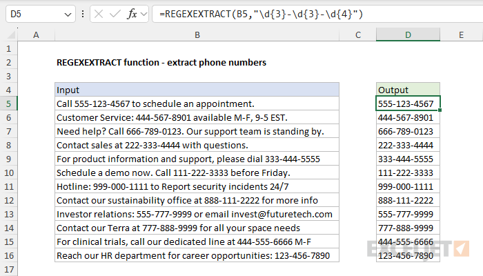
The REGEXEXTRACT function extracts text matching a specific regex pattern from a given text string. For the advanced Excel user, this function is a major upgrade. Instead of working out complex formulas based on functions like LEFT, RIGHT, FIND, and MID, REGEXEXTRACT can target data very precisely with a single regular expression (regex) pattern. With REGEXEXTRACT, you can easily extract numbers, dates, times, email addresses, and other text with a recognizable structure. REGEXEXTRACT not only saves time but also reduces errors created by complicated workarounds.
Learn more about the REGEXEXTRACT function.
REGEXREPLACE function
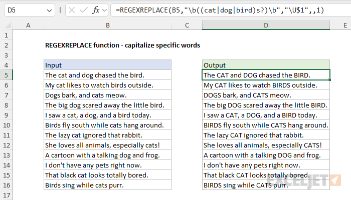
The REGEXREPLACE function replaces text that matches a specific regular expression (regex) pattern in a given text string. You can think of REGEXREPLACE as a much more powerful version of the simplistic SUBSTITUTE function. While both functions can be used to search and replace simple text strings, REGEXREPLACE can use regex, a powerful language built for matching and manipulating text values. This function is a major upgrade to Excel's rather primitive text-replacement functions.
Learn more about the REGEXREPLACE function.
REGEXTEST function
REGEXTEST brings the power of regular expressions to ordinary Excel formulas. It tests whether a text string matches a specific pattern, returning TRUE or FALSE. This versatile function can validate email addresses, check for specific number formats, or search for complex text patterns. For instance, =REGEXTEST(A1,"[0-9]") will return TRUE if cell A1 contains any numeric digit, and =REGEXTEST(A1,"[A-Z]" will return TRUE if A1 contains any uppercase letters. REGEXTEST opens up new possibilities for data validation and text analysis directly within Excel formulas. You can even combine REGEXTEST with other functions like IF and FILTER to implement very sophisticated logic.
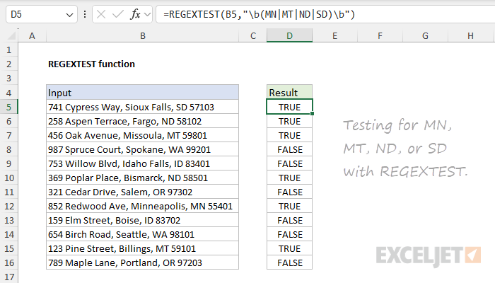
Learn more about the REGEXTEST function.
New Excel 365 functions
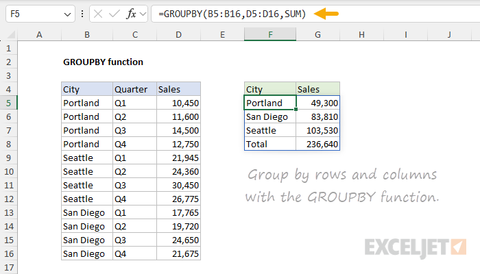
GROUPBY function
GROUPBY is Excel's answer to how to make a simple Pivot Table with a formula. It creates a dynamic summary table with a single formula, similar to a Pivot Table, but without formatting. For instance, you could use =GROUPBY(B5:B16,D5:D16,SUM) to summarize sales by city, where B5:B16 contains city names, and D5:D16 contains sales amounts. Unlike a Pivot Table, which needs to be refreshed, The summary returned by the GROUPBY function is fully dynamic and will immediately recalculate when source data changes. GROUPBY is particularly useful when you need a quick, dynamic summary without the overhead of a full Pivot Table.
Learn more about the GROUPBY function.
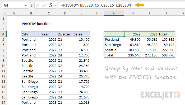
PIVOTBY function
Like the GROUPBY function, PIVOTBY can create a Pivot Table with a formula. The difference is that PIVOTBY can perform two-dimensional grouping by row and column, whereas GROUPBY can group by row only. For example, =PIVOTBY(B5:B28,C5:C28,E5:E28,SUM) will summarize sales by city (in rows) and year (in columns), where B5:B28 contains city names, and C5:C16 contains years. This function is powerful for users who want the layout of a pivot table combined with the flexibility and precision of a formula. It's an excellent tool for creating dynamic, formula-based summaries that update automatically when source data changes.
Learn more about the PIVOTBY function.
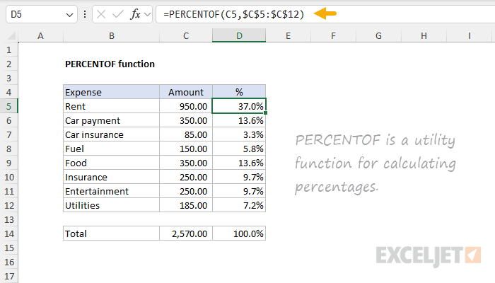
PERCENTOF function
PERCENTOF calculates the percentage of a subset of data relative to all data. It's a handy shortcut for common percentage calculations, returning a decimal that can be formatted as a percentage in Excel. For example, =PERCENTOF(250,1000) returns 0.25, which, when formatted as a percentage, displays as 25%. This function is useful in any scenario where you need to express a part-to-whole relationship. Although you can use PERCENTOF as a standalone function, it was introduced as a companion to GROUPBY and PIVOTBY to make it easy to incorporate "percentage of" calculations into formula-based pivot tables.
Learn more about the PERCENTOF function.
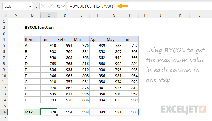
BYCOL function
BYCOL is one of two new functions in Excel (BYROW is the other) that let you apply aggregate calculations "by column" or "by row" in a single formula step. Specifically, BYCOL applies a LAMBDA function to each column in an array, returning one result per column as a single array. The concept may seem abstract, but in practice, BYCOL is quite useful. For instance, assume you have 6 columns of numbers in C5:H14. This formula will return the maximum value in each of the 6 columns in one step: =BYCOL(C5:H14,MAX). BYCOL runs on every column, returning a single result for each. Since it can apply custom LAMBDA logic, BYCOL can perform operations far beyond simple sums or averages.
Learn more about the BYCOL function.
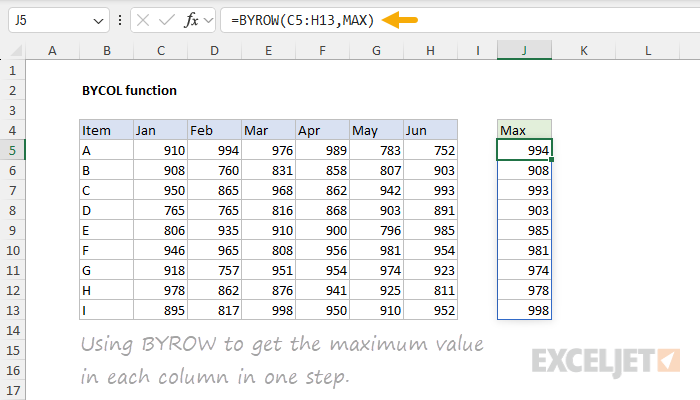
BYROW function
BYCOL is the companion to the BYROW function. The purpose of BYROW is to process data in an array or range in a "by row" fashion. Specifically, BYCOL applies a LAMBDA function to each row in an array, returning one result per row in a single step. If BYROW is given an array with 100 rows, BYROW will return 100 results. The calculation performed on each row is flexible. For example, if you have 9 rows of data in 6 columns as below, you can use a formula like this to get the maximum value in each row: =BYROW(C5:H13,MAX). The result is all 9 maximum values in one step. BYROW runs on each row, returning a single result for each.
Learn more about the BYROW function.
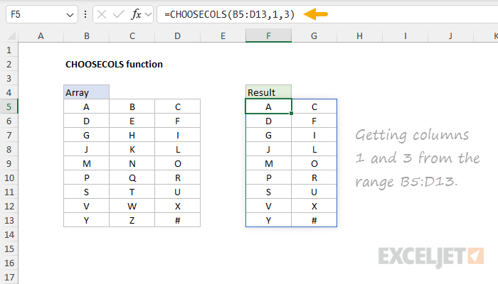
CHOOSECOLS function
CHOOSECOLS selects specific columns from an array or range by position. The columns to return are provided as numbers. For example, you can ask for the first, third, and fifth columns with a formula like =CHOOSECOLS(range,1,3,5). CHOOSECOLS is particularly useful when working with structured data where row positions have specific meanings. In addition to bringing together desired columns, you can also think of CHOOSECOLS as a great way to quickly discard unwanted columns. One interesting use of CHOOSECOLS is to create a mini-dashboard. The result from CHOOSECOLS is always a single array that spills onto the worksheet.
Learn more about the CHOOSECOLS function.
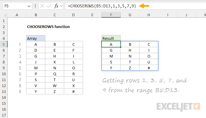
CHOOSEROWS function
CHOOSEROWS works like the CHOOSECOLS function. However, whereas CHOOSECOLS fetches specific columns, CHOOSEROWS fetches specific rows. For example, you could get the first, third, and fifth row from a range with a formula like =CHOOSEROWS(range,1,3,5). CHOOSEROWS is especially handy when working with structured data where row positions have meaning, like days of a week, days of a month, or hours in a day. The result from CHOOSEROWS is always a single array that spills onto the worksheet.
Learn more about the CHOOSEROWS function.
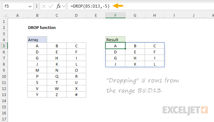
DROP function
The DROP function returns a subset of a given array by "dropping" rows and columns. Rows and columns can be dropped from the start or end of the given array. For example, you could "drop" the last three rows from a range with a formula like =DROP(range,-3). DROP complements the TAKE function. Whereas TAKE selects specific rows or columns from a range, DROP removes specific rows or columns from a range or array. DROP is useful for removing headers, trimming datasets, or whenever you want to reduce the size of a range by removing rows and/or columns.
Learn more about the DROP function.
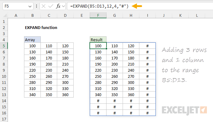
EXPAND function
As the name suggests, EXPAND increases the size of an array by adding rows, columns, or both. You can specify what value to fill the new cells with, making it useful for "padding" arrays or preparing data for operations that require specific dimensions. The values given for rows and columns represent the dimensions of the final array, not the number of rows or columns to add. For instance, =EXPAND(A1:B2,4,3,"N/A") would expand a 2x2 array to a 4x3 array, filling new cells with "N/A". This function is particularly useful in scenarios where you need to standardize the size of datasets or create placeholder structures for data input.
Learn more about the EXPAND function.
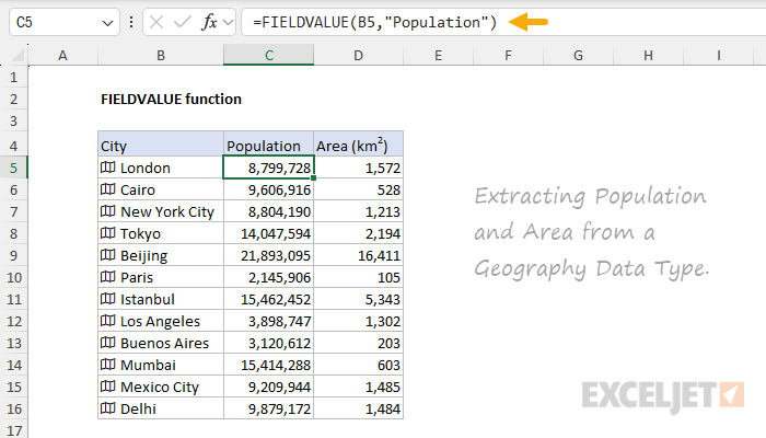
FIELDVALUE function
FIELDVALUE is a utility function designed specifically for Excel's data types, such as stocks, geography, or currency. As implied by the name, FIELDVALUE returns a specific field value from a Data Type. For example, with a stock data type in cell A1, you can request the last close price with a formula like this: =FIELDVALUE(A1,"previous close"). FIELDVALUE is an alternative to the "dot" syntax: =A1.[Previous close]. The main advantage of using FIELDVALUE is the ability to specify a field value as plain text, which can be more convenient in a formula.
Learn more about the FIELDVALUE function.
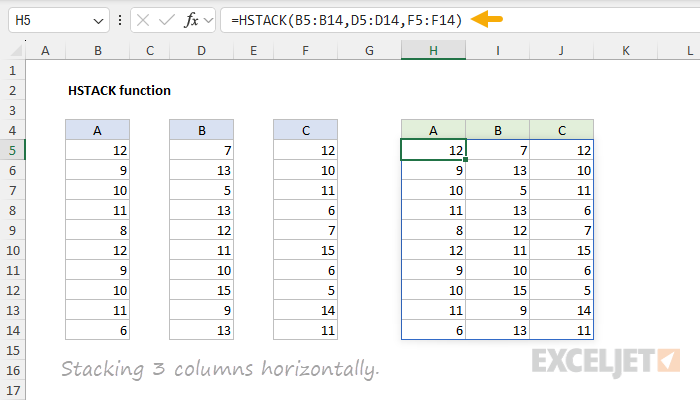
HSTACK function
HSTACK combines arrays or ranges horizontally into a single array. Each subsequent array is appended to the right of the previous array. For example, =HSTACK(A1:A10,C1:C10) would combine two columns with 10 rows each into a single range with two columns and 10 rows. This function is particularly useful when you need to merge data from different sources or expand your dataset with additional columns of information. The output from HSTACK is fully dynamic. If data changes, the result from HSTACK will be updated immediately. HSTACK is closely related to VSTACK. Use HSTACK to combine ranges horizontally and VSTACK to combine ranges vertically.
Learn more about the HSTACK function.
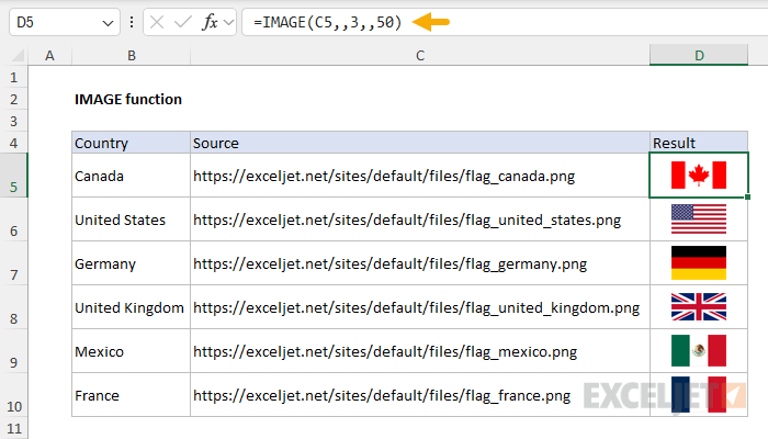
IMAGE function
The IMAGE function is Excel's solution for adding online images to a worksheet with a formula. As long as the image is available online and reachable via the "https://" protocol, IMAGE will fetch the image and bring a copy of it into a cell on the worksheet. You can use the IMAGE function to add images to things like employee lists, product information, games, and other data that includes images. Of course, you can manually insert an image into a cell anytime, so why use IMAGE? I think the main use case for IMAGE is importing a larger number of images with a formula that calculates the path to each image automatically. It might not matter much for 10 images, but for 100 images or a thousand, this is a big upgrade.
Learn more about the IMAGE function.
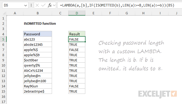
ISOMITTED function
ISOMITTED is a specialized function designed to work with LAMBDA functions. Its purpose is to provide a way to make LAMBDA arguments optional. ISOMITTED checks whether an optional argument in a LAMBDA function has been provided or not. For instance, you can use ISOMITTED in a custom LAMBDA function like this: =LAMBDA(a,[b],IF(ISOMITTED(b),a+10,a+b)). Although this formula takes two arguments, a and b, b is optional since it is enclosed in square brackets. Inside the LAMBDA, ISOMITTED checks for b. If b is omitted, the formula returns a+ 10. If b is provided, the formula returns a + b. In summary, ISOMITTED is a helper function that allows LAMBDA functions with optional arguments to alter behavior based on what arguments are provided.
Learn more about the ISOMITTED function.
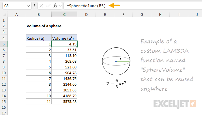
LAMBDA function
The LAMBDA function allows you to create custom, reusable functions directly in Excel without VBA or macros. For example, you could create a simple squaring function with =LAMBDA(x,x^2). Once defined and named, a LAMBDA function can be used anywhere in your workbook. This powerful feature lets you define complex operations once and reuse them throughout your workbook, significantly reducing redundancy since there is just one copy of code to maintain. LAMBDA functions can range from simple calculations to complex, multi-step operations, opening up new possibilities for customizing Excel to your specific needs. LAMBDA functions can also appear inside many other new functions (i.e. BYCOL, BYROW, MAP, SCAN, REDUCE, etc.) that loop over arrays and apply calculations.
Learn more about the LAMBDA function.
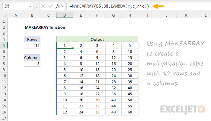
MAKEARRAY function
MAKEARRAY is a custom array generator. It creates an array with specified dimensions, filling it with values defined by a custom LAMBDA formula. For example, =MAKEARRAY(5,5,LAMBDA(r,c,r*c)) would create a 5x5 multiplication table. This function is useful for creating complex arrays, generating test data, or performing element-wise operations across a grid of values. It's particularly handy when you need arrays with calculated values that follow a specific pattern or rule. Note the related RANDARRAY function can create a custom-sized array containing random numbers.
Learn more about the MAKEARRAY function.
MAP function
MAP brings a fundamental concept from functional programming to Excel. It applies a custom operation to each cell in a range, and returns an array of results. It's a bit like a custom mini-function that runs on every cell. For instance, =MAP(A1:E10,LAMBDA(x,x*2)) would double each number in the range A1:E10. MAP is especially good when you want to process each element in an array using functions like AND and OR. Normally, functions like this break array formulas because they aggregate multiple values into a single value. However, because MAP operates on one cell at a time, it works. MAP is versatile, allowing you to transform data, combine information from multiple ranges, and perform complex calculations on a cell-by-cell basis across ranges of data.
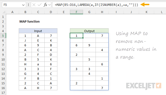
Learn more about the MAP function.
REDUCE function
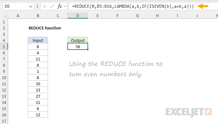
The REDUCE function applies a custom LAMBDA function to each element in a given array and accumulates results to a single value. REDUCE is useful for iterative calculations where each step depends on the result of the previous step and uses a different input value. For example, you can use the REDUCE function to calculate conditional sums and counts, similar to SUMIFS and COUNTIFS, but with more flexibility. For example, to calculate the sum of all numbers in A1:E10, you can use a formula like =REDUCE(0,A1:E10,LAMBDA(a,v,a+v)). To calculate the sum of all odd numbers, you can use a formula like =REDUCE(0,A1:E10,LAMBDA(a,v,IF(ISODD(v),a+v,a))).
Learn more about the REDUCE function.
SCAN function
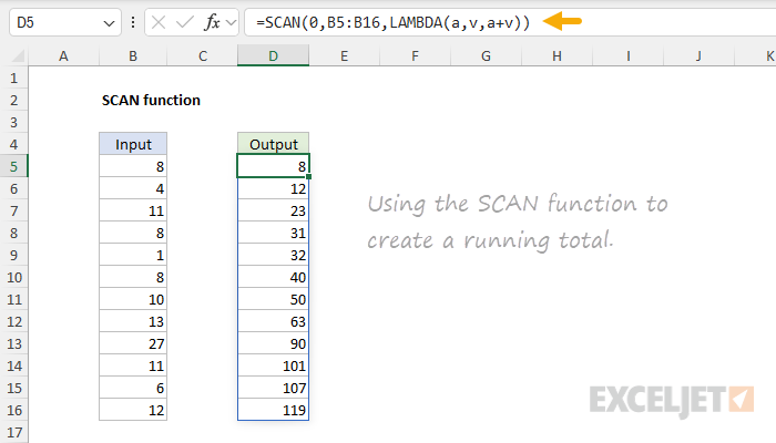
The SCAN function iterates through the elements in an array with custom logic and returns an array that contains the intermediate values created during the scan. SCAN is similar to REDUCE, but instead of producing a single result, it returns an array of intermediate results. It's like getting the play-by-play of a cumulative calculation at each step. This function is particularly useful for creating running totals, running counts, and the results from other cumulative calculations. For example, to create a running total of the numbers in A1:A10 you can use SCAN like this: =SCAN(0,A1:A10,LAMBDA(a,v,a+v)). To create a running total of odd values only, you can use =SCAN(0,A1:A10,LAMBDA(a,v,IF(ISODD(v),a+v,a))).
Learn more about the SCAN function.
STOCKHISTORY function
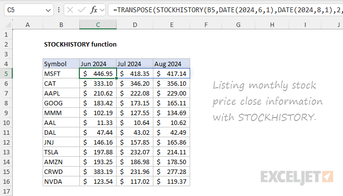
The STOCKHISTORY function retrieves historical stock price information based on a given stock symbol and date range. This function saves you from manual data entry or importing external data, allowing you to perform stock analysis and financial modeling directly within Excel using up-to-date market information. Although the name suggests that STOCKHISTORY is meant to work only with stocks, STOCKHISTORY can also work with bonds, index funds, mutual funds, and currency exchange rates. Note that STOCKHISTORY only returns historical information recorded after the market closes. It does not return real-time data.
Learn more about the STOCKHISTORY function.
TAKE function
TAKE extracts a specific number of rows or columns from an array, either from the beginning or the end. It's like a data slicer for ranges. For instance, =TAKE(A1:C100,10) would return the first 10 rows from the range, while =TAKE(A1:C100,-10) would return the last 10 rows. This function is particularly useful when you need to work with a subset of your data, like the top n rows or the last n columns, without altering the original dataset. TAKE is also great for creating dynamic ranges that adjust based on the data. For example, if you configure TAKE to return the last 7 rows in a table, it will continue to update as more rows are added. Note that the TAKE function is related to the DROP function, which removes rows and/or columns from a range.
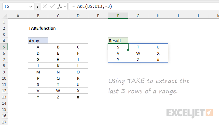
Learn more about the TAKE function.
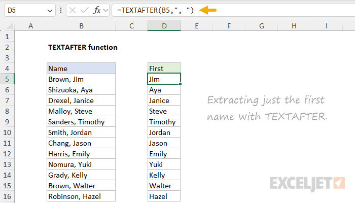
TEXTAFTER function
TEXTAFTER splits a text string and extracts the portion of a string that comes after a given delimiter. It's designed to work with structured text with a clear pattern and delimiter. For example, =TEXTAFTER("john.doe@example.com","@") will return the email domain, "example.com". TEXTAFTER can handle multiple delimiters and be configured to extract text after the "nth instance" of a given delimiter, making it very useful for parsing emails, names, URLs, and other text with delimiters. Compared to older, more complicated solutions, TEXTAFTER greatly simplifies the process of splitting text strings.
Learn more about the TEXTAFTER function.
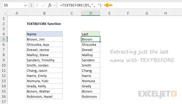
TEXTBEFORE function
TEXTBEFORE is the counterpart to TEXTAFTER. It extracts the portion of a string that comes before a specified delimiter. For instance, =TEXTBEFORE("john.doe@example.com","@") will return "john.doe". TEXTBEFORE can be configured to extract text after a specific instance of a delimiter (i.e. after the second space). You can even use TEXTBEFORE together with TEXTAFTER to perform more specific text extraction. Like TEXTAFTER, it offers options for handling multiple delimiters and case sensitivity.
Learn more about the TEXTBEFORE function.
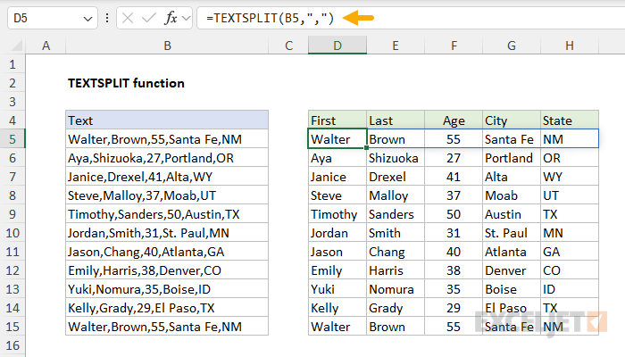
TEXTSPLIT function
Whereas TEXTAFTER and TEXTBEFORE return the text before or after a delimiter, TEXTSPLIT splits text at a delimiter and returns all the parts in one go. The output from TEXTSPLIT is an array that will spill into multiple cells in the workbook. For example, =TEXTSPLIT("apple,banana,cherry",",") would return an array with three cells containing "apple", "banana", and "cherry". This function is incredibly useful for parsing structured text data, converting delimited strings into usable Excel ranges, or converting complex text structures into manageable pieces.TEXTSPLIT can handle multiple delimiters and even different delimiters for rows and columns.
Learn more about the TEXTSPLIT function.
TOCOL function
TOCOL transforms a two-dimensional array into a single column. It's like flattening your data vertically. For instance, =TOCOL(B5:D8) would take a 4x3 grid and turn it into a single column with 12 cells. This function can scan values "by row" or "by column" and offers options to ignore empty cells and errors. TOCOL is particularly useful when you need to restructure data: create lists from tables, prepare data for vertical analysis, or simplify data going into other functions.
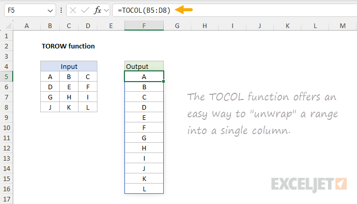
Learn more about the TOCOL function.
TOROW function
TOROW is the horizontal counterpart to TOCOL. It transforms a two-dimensional array into a single row, essentially flattening data horizontally. For example, =TOROW(B5:D8) will take a 4x3 grid and return a single row with 12 cells. Like TOCOL, it offers options to scan by row or column and can ignore blanks or errors. This function is helpful whenever you need to reshape data in a 2D range or array into a horizontal format with one row.
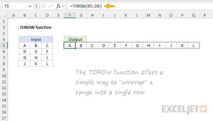
Learn more about the TOROW function.
ARRAYTOTEXT function
You might not know that Excel deals with ranges internally as "arrays", which have a particular syntax when displayed as text. The classic way to "see" this syntax in Excel is to use the F9 key when investigating a formula. But what if you want to show this syntax directly on the worksheet? ARRAYTOTEXT is a utility function that lets you format the values in a range in array syntax. It converts an array or range into a text string that can be displayed directly on the worksheet. Unless you are deep in the weeds of array formulas, you probably don't need to worry about this function.
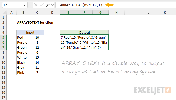
Learn more about the ARRAYTOTEXT function.
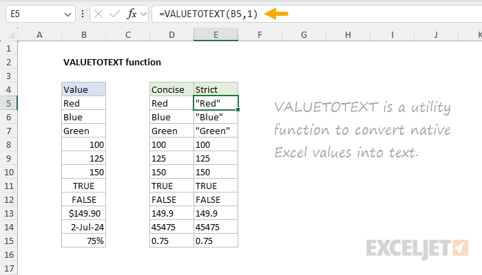
VALUETOTEXT function
VALUETOTEXT is a utility function that converts various types of values (numbers, dates, booleans, etc.) into their text representations. For instance, =VALUETOTEXT(42) would return "42" as text, and =VALUETOTEXT(TRUE) would return "TRUE". By default, text values pass through unaffected, while other values are quoted. However, in strict mode, text values are enclosed in double quotes ("").
Learn more about the VALUETOTEXT function.
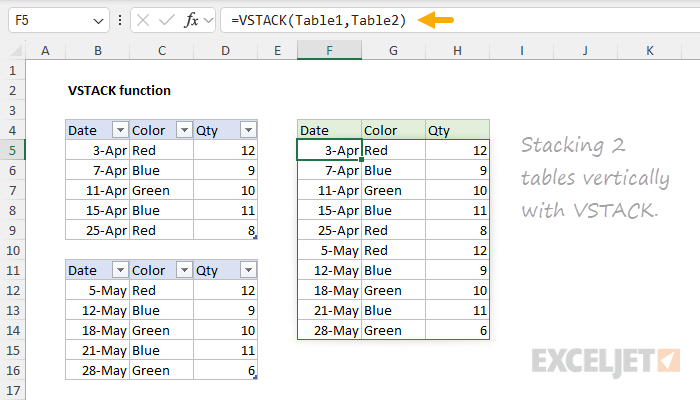
VSTACK function
VSTACK is the vertical counterpart to the HSTACK function. While HSTACK stacks ranges horizontally, VSTACK stacks ranges vertically, one on top of another. For example, =VSTACK(A1:A5,C1:C5) will combine the two columns into a single column of 10 cells. This function is particularly useful when you need to combine data from different sources, for example, data on different sheets. It is also handy when you want to attach headers to calculation results inside a formula. VSTACK can handle ranges of different widths, making it a flexible way to handle different data combination scenarios. The output from VSTACK is dynamic and will immediately update if source data changes.
Learn more about the VSTACK function.
WRAPCOLS function
WRAPCOLS takes a one-dimensional array (i.e. a single row or column) and wraps it into multiple columns based on a specified number of rows. WRAPCOLS works one column at a time using a given "wrap count" to determine when to start a new column. For instance, =WRAPCOLS(B5:B16,4) will arrange the 12 values in B5:B16 into a table with 4 rows and 3 columns. WRAPCOLS is useful when you need to reshape linear data into a table working "by column". It can also be used to re-wrap data previously unwrapped by the TOCOL or TOROW function.

Learn more about the WRAPCOLS function.
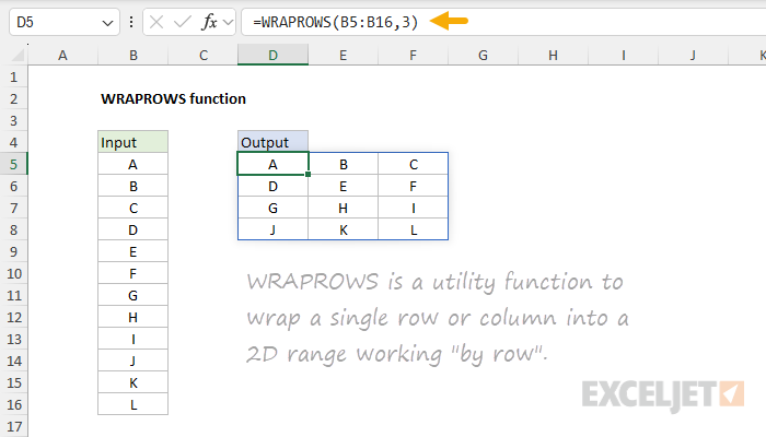
WRAPROWS function
WRAPROWS is the row-wise version of WRAPCOLS. It takes a one-dimensional array (i.e. a single row or column) and wraps it into multiple rows based on a specified number of columns. WRAPROWS works one row at a time, adding values until it hits a given "wrap count", then beginning a new row. For example, =WRAPROWS(B5:B16,4) will take 12 cells in B5:B16 and arrange them into a table with 4 rows and 3 columns. WRAPCOLS is useful when you want to wrap linear data into a table, working one row at a time.
Learn more about the WRAPROWS function.
New Excel 2021 functions
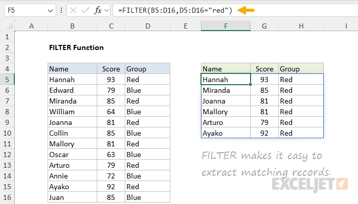
FILTER function
A true game-changer, the FILTER function "filters" data based on one or more conditions and extracts matching values. The result from FILTER is an array of matching values from the original data. The results from FILTER are dynamic. If source data changes or if conditions are modified, FILTER will return new results. This makes FILTER an excellent way to isolate and inspect specific data without altering the original dataset. For example, =FILTER(B5:D16,D5:D16="red") will return all rows in B5:D16 where the color in column D is "Red", as seen below. FILTER is highly versatile. You can filter data that occurs in a certain year or month, find data between two values, and isolate records that contain specific text. FILTER can even filter columns.
Learn more about the FILTER function.
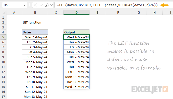
LET function
LET brings local variables to Excel formulas. It allows you to assign names to intermediate calculations within a formula, making complex formulas more readable and efficient. For instance, =LET(x,A1+A2, y,B1+B2, x*y) assigns names to two calculations and then uses them in a final calculation. These variables are temporary and live only in your formula. LET can significantly improve performance by eliminating redundant calculations. LET can radically simplify more complex formulas that reuse intermediate results or ranges multiple times.
Learn more about the LET function.
RANDARRAY function
RANDARRAY is an on-demand random number generator. It creates an array of random numbers with specified dimensions. For example, RANDARRAY(10) will generate 10 random decimal values in a column, and =RANDARRAY(5,3,1,100,TRUE) generates a 5x3 array of random integers between 1 and 100. RANDARRAY is useful for random sorts, random sampling, and for creating test data from randomly selected values. You can also use RANDARRAY to generate random text strings and a random list of names.
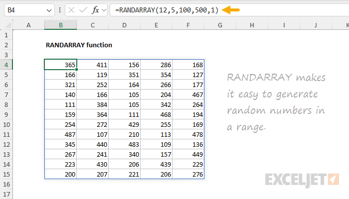
Learn more about the RANDARRAY function.
SEQUENCE function
SEQUENCE is a function for generating sequential numbers. For instance, =SEQUENCE(10) returns the numbers 1-10 in an array that spills into a single column. SEQUENCE has options for the dimensions of the final array, and for the start value and step size. For example, =SEQUENCE(12,5,0,5) creates a 12x5 array of numbers starting at zero and incrementing by 5, as seen in the worksheet below. This function is useful for generating numbered lists, creating row or column numbers, or providing sequential input to other formulas. SEQUENCE can be used to create date ranges, sequential months and years, and in other situations where you need sequential numbers.
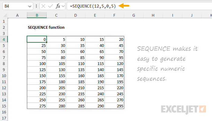
Learn more about the SEQUENCE function.
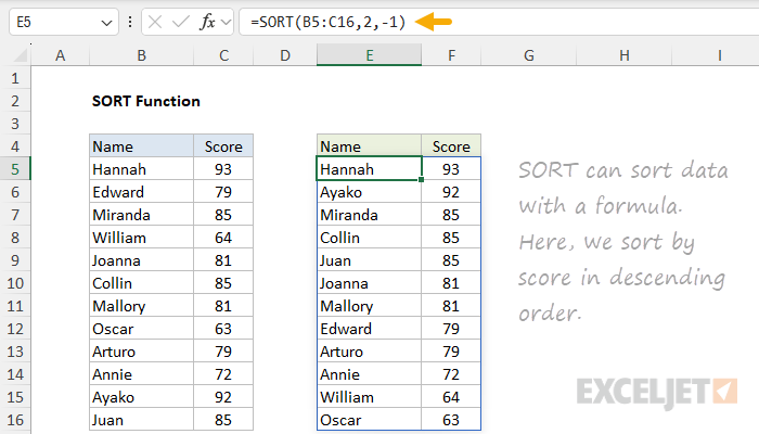
SORT function
SORT brings the power of sorting directly into your formulas. It can sort data in ascending or descending order and can sort by more than one column. For example, =SORT(B5:C16,2,-1) sorts the range B5:C16 based on the values in column C in descending order. The result is a dynamic array that updates automatically when source data changes. This function allows for real-time sorting without altering the original data, making it ideal for creating sorted views for reporting. SORT is especially useful in dashboards or reports where you want to highlight top or bottom performers in a set of data.
Learn more about the SORT function.
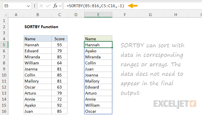
SORTBY function
SORTBY takes sorting to the next level by allowing you to sort data based on values in corresponding ranges or arrays. This means you can sort using values that don't appear in the final result. For instance, =SORTBY(B5:C16,C5:C16) sorts the names in column B based on the scores in column B, as seen below. Like the simpler SORT function, SORTBY can sort by more than one column in ascending or descending order. This function is especially useful when you need to sort data in a custom order.
Learn more about the SORTBY function.
UNIQUE function
The UNIQUE function is another game-changer, making many complex formulas of the past obsolete. As the name suggests, UNIQUE extracts a list of unique values from a range or array. The result is a dynamic array of unique values: if source data changes, UNIQUE will continue to output the latest unique values. For example, the formula =UNIQUE(B5:B16) returns a list of the 4 unique colors in B5:B16, as seen below. This function is useful for identifying unique entries in a dataset, for creating category lists, and for cleaning up data. It can also be used to generate the values used in dropdown lists.
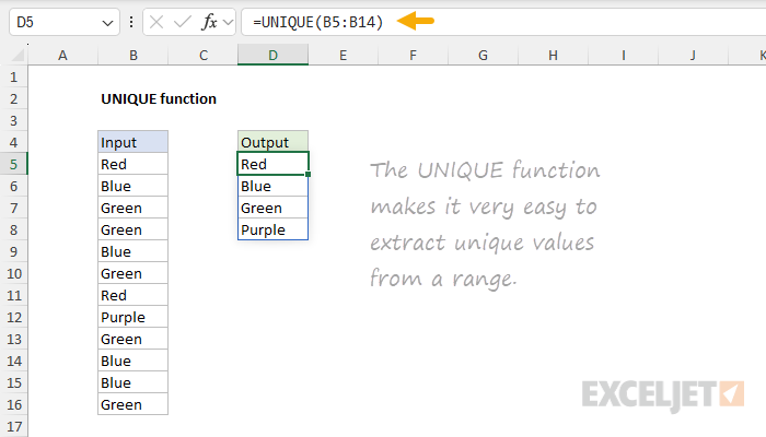
Learn more about the UNIQUE function.
XLOOKUP function
XLOOKUP is a modern successor to VLOOKUP and HLOOKUP. It is a flexible and versatile function that can be used in a wide variety of situations. XLOOKUP can find values in vertical or horizontal ranges, can perform approximate and exact matches, and supports wildcards (* ?) for partial matches. In addition, XLOOKUP can perform a reverse search and offers a super-fast binary search option when working with large datasets. XLOOKUP simplifies many lookup scenarios that previously required complex combinations of functions, making data retrieval more intuitive and flexible. Whether you are just getting started with Excel or are already a heavy user, XLOOKUP should be your go-to solution for most lookup problems. Note: if you after multiple results, see the FILTER function.
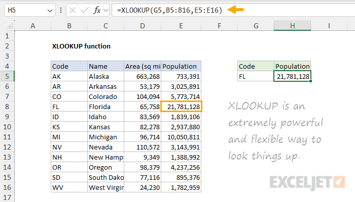
Learn more about the XLOOKUP function.
XMATCH function
XMATCH is the modernized version of the MATCH function. Like MATCH, it performs a lookup and returns the numeric position of the lookup value as a result, which is usually handed off to the INDEX function to retrieve a value. However, XMATCH offers a number of new features that bring it up to speed with XLOOKUP: it defaults to an exact match, it can match the next smaller or next larger, it can perform a reverse search, and it offers a super fast binary search for large data sets. Best of all, you can use XMATCH as a drop-in replacement for MATCH in most cases. In the worksheet below, XMATCH is used with INDEX to look up annual sales for the car manufacturer entered in cell G4.
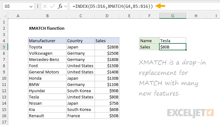
Learn more about the XMATCH function.
New 2019 functions
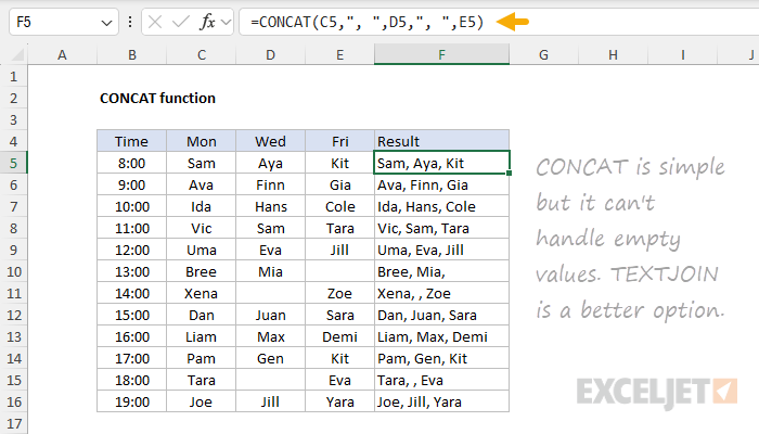
CONCAT function
CONCAT is a modernized version of the CONCATENATE function. Like CONCATENATE, it can join text from multiple cells without a delimiter. Unlike its predecessor, CONCAT will accept a range of cells to join, in addition to individual cell references. You can see a basic example of CONCAT below used to join the names in columns C, D, and E with commas and spaces (", "). However, note that CONCAT has no setting to ignore empty values and no way to supply a delimiter as an argument. For these reasons, I recommend you ignore CONCAT and use the TEXTJOIN function instead, which is far more capable.
Learn more about the CONCAT function.
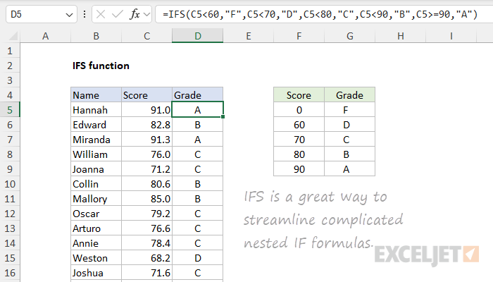
IFS function
IFS simplifies the process of testing multiple conditions in Excel. It allows you to evaluate several logical tests and return a value corresponding to the first TRUE result. Think of it as a more efficient alternative to nested IF statements. For example, =IFS(C5<60,"F",C5<70,"D",C5<80,"C",C5<90,"B",C5>=90,"A") assigns letter grades based on numeric scores in column C, as seen in the worksheet below. IFS makes complex conditional logic more readable and manageable. It's great for grading systems, categorization tasks, or any scenario where you need to evaluate multiple conditions in a specific order. You can use the IFS function when you want a self-contained formula to test multiple conditions at the same time without nesting multiple IF statements.
Learn more about the IFS function.
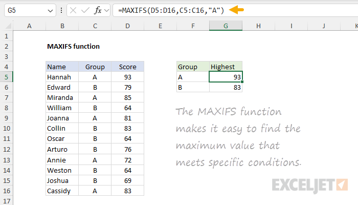
MAXIFS function
MAXIFS finds the largest value among cells that meet multiple criteria. It's like combining the MAX function with multiple condition checks. This function is useful in scenarios where you need to find the highest value that meets one or more specific conditions, such as the highest value in a given group. For example, =MAXIFS(D5:D16,C5:C16,"A") finds the maximum value in column D where the group in column C is "A". MAXIFS is a handy tool for all kinds of data analysis.
Learn more about the MAXIFS function.
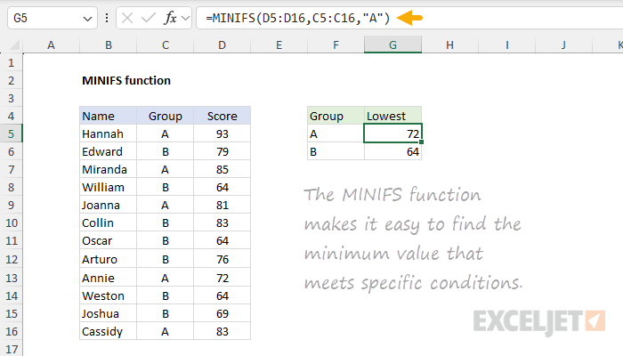
MINIFS function
MINIFS is the counterpart to MAXIFS, finding the smallest value that meets multiple criteria. Like MAXIFS, it combines the functionality of MIN with conditional filtering. For instance, =MINIFS(D5:D16,C5:C16,"A") finds the minimum value in column D where the group in column C is "A". This function is helpful in situations such as identifying the lowest price for products meeting certain specifications or finding the minimum value within a specific subset of your data. MINIFS is particularly valuable in pricing analysis, performance management, or any scenario where you need to identify the lowest value that meets multiple conditions.
Learn more about the MINIFS function.
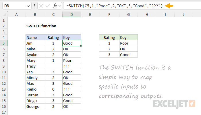
SWITCH function
SWITCH is like a streamlined IF-THEN-ELSE statement for Excel. It compares a single expression against a list of values and returns the result corresponding to the first match. For instance, =SWITCH(C5,1,"Poor",2,"OK",3,"Good","???") categorizes numeric ratings in column C with the categories "Poor", "OK", and "Good". Unrecognized ratings default to "???". This function simplifies formulas that would otherwise require nested IF statements, especially when dealing with discrete values or categories. SWITCH is particularly useful for mapping a limited number of specific inputs to corresponding outputs in a simple all-in-one formula.
Learn more about the SWITCH function.
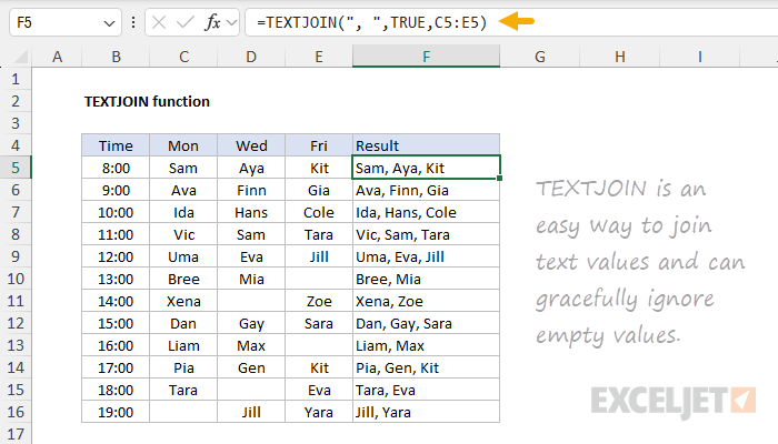
TEXTJOIN function
TEXTJOIN is the sophisticated cousin of CONCAT. It concatenates multiple text strings, ranges, or constants, with the added flexibility of specifying a delimiter to use between each item. For example, =TEXTJOIN(", ",TRUE,C5:E5) joins the text in C5:E5, separated by commas, while ignoring empty cells. Because TEXTJOIN can ignore empty cells, it is more versatile than the CONCAT function. This function is particularly useful for creating comma-separated lists and other delimited text strings.