FILTER Function

The FILTER function "filters" data based on one or more conditions, and extracts matching values. The conditions are provided as logical expressions that test the source data and return TRUE or FALSE. The result from FILTER is an array of matching values from the original data. The results from FILTER are dynamic: if source data changes, or if conditions are modified, FILTER will return new results. Because FILTER returns a dynamic array, results spill onto the worksheet automatically and stay in sync as the data changes. This makes FILTER a very good way to isolate and inspect specific data without altering the original dataset. Watch the video below to see a quick example of FILTER in action:

FILTER is a flexible function that can extract matching data based on a wide variety of conditions. If you can write a logical test that returns TRUE or FALSE, you can use that test to extract data with FILTER. You can filter data that occurs in a certain year or month, data associated with a particular day of the week, data that contains specific text, data that meets a numeric threshold, and more.

Key features

• Extracts records that meet one or more conditions
• Returns a dynamic array that spills onto the worksheet and updates automatically
• Criteria are supplied as one or more logical tests that return TRUE or FALSE
• Combine conditions with Boolean logic: multiply (*) for AND, add (+) for OR
• Optional if_empty argument returns a custom result when nothing matches
• Works with both vertical and horizontal data
• Pairs naturally with SORT, UNIQUE, and other dynamic array functions
• Returns a #CALC! error when no records meet supplied conditions

Table of contents

• Basic examples
• Extract values greater than 100
• Filter by a single condition
• Filter with multiple criteria
• Filter this OR that
• Filter between two dates
• Filter where text contains
• Filter top N values
• Filter and sort
• Filter horizontal data
• Complex multiple criteria
• Notes

Basic examples

The FILTER function takes two required arguments: array and include. The array is the source data to filter, and include is one or more logical tests that return TRUE or FALSE for each row (or column) in the array. The examples below show the basic pattern. In each case, range is a stand-in for the actual cells on your worksheet:

=FILTER(range,range>100)                  // numbers over 100
=FILTER(range,range="red")                // text equals "red"
=FILTER(range,range="red","No results")   // message when nothing matches
=FILTER(range,(range1="red")*(range2>80)) // condition1 AND condition2
=FILTER(range,(range1="a")+(range2="b"))  // condition1 OR condition2

When you combine conditions, each logical expression must return an array with dimensions that match the array argument. The examples below show how these patterns work in real worksheets.

Extract values greater than 100

In the worksheet below, the goal is to extract the values in B5:B16 that are greater than 100. The formula in cell D5 is:

=FILTER(B5:B16,B5:B16>100)

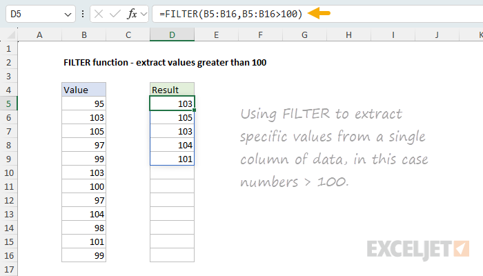
The include argument is the logical expression B5:B16>100. Because there are 12 cells in the range, this expression returns an array of 12 TRUE and FALSE values, one for each value in B5:B16:

=FILTER(B5:B16,{FALSE;TRUE;TRUE;FALSE;FALSE;TRUE;FALSE;FALSE;TRUE;FALSE;TRUE;FALSE})

Each result in the array corresponds to a value in B5:B16. FILTER uses this array to "filter" the data: values associated with TRUE are returned, and values associated with FALSE are discarded. The five values greater than 100 spill into the range D5:D9. Because the result is dynamic, editing any number in B5:B16 immediately updates the output.

For more information about how arrays are used in Excel formulas see: Arrays in Excel.

Filter by a single condition

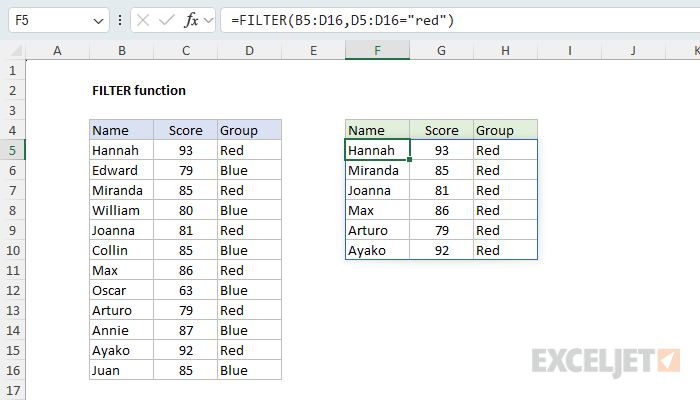
In the example below, the goal is to extract all rows where the Group is "Red". The data is in the range B5:D16, and the formula in cell F5 is:

=FILTER(B5:D16,D5:D16="red")

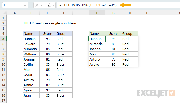
Here, the array is the full table in B5:D16, and include is the logical expression D5:D16="red", which tests the Group column. Text comparisons in Excel are not case-sensitive, so "red", "Red", and "RED" are treated the same. The expression returns TRUE for each row in the Red group and FALSE for the rest, and FILTER returns all three columns (Name, Score, and Group) for the matching rows. The six matching records spill into the range F5:H10.

You can also place the group condition in a cell so the result updates when you type a new group. For example, with a group name like "Red" entered in cell H2, the include argument would become D5:D16=H2. When you change H2 to "Blue", FILTER will return a new set of records.

Filter with multiple criteria

At first glance, it is not obvious how to apply more than one condition with FILTER. Unlike older functions like COUNTIFS and SUMIFS, which provide separate arguments for each condition, FILTER has just one include argument. The trick is to build a single logical expression with Boolean logic. In the worksheet below, the goal is to extract rows where the Group is "Red" AND the Score is at least 85. The formula in cell F5 is:

=FILTER(B5:D16,(D5:D16="red")*(C5:C16>=85))

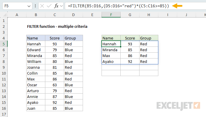
The two conditions are joined with the multiplication operator (*), which creates AND logic: a row is included only when both expressions are TRUE. This works because the math forces TRUE and FALSE into 1 and 0, so the product is 1 (TRUE) only when every condition is 1. The four matching records spill into the range F5:H8.

For more details, see Filter with multiple criteria. For a brief overview of how Boolean algebra can be used in Excel for operations like AND or OR, watch this video: Boolean algebra in Excel.

Filter this OR that

To extract data that meets one condition OR another, use addition (+) instead of multiplication. In the example below, the goal is to return all rows where the Group is either "A" or "C". The formula in cell F5 is:

=FILTER(B5:D16,(D5:D16="A")+(D5:D16="C"))

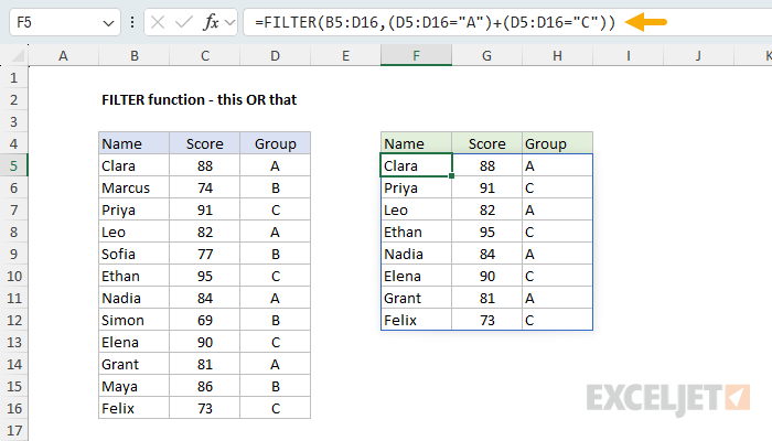
Addition creates OR logic: when the results of the two expressions are added together, the total is 1 or more (TRUE) if either condition is met, and 0 (FALSE) only when both fail. FILTER returns every row in Group A or Group C, which spills into the range F5:H12. You can extend this same approach to apply more conditions by adding more logical expressions, joined with (*) or (+) as appropriate.

For more details, see Filter this OR that.

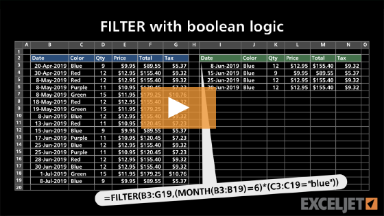
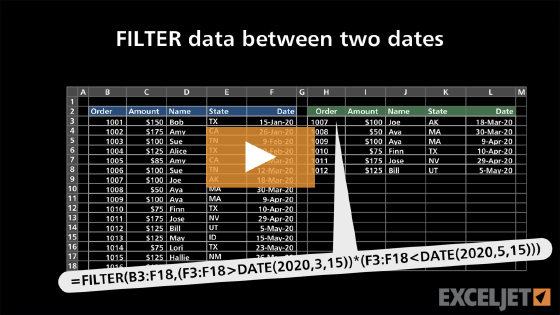
Filter between two dates

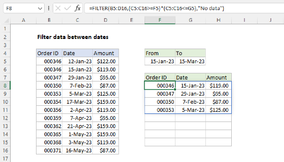
FILTER works with dates by building logical tests that operate on Excel dates. In the worksheet below, the goal is to extract orders with a date between a start date in F5 and an end date in G5. The formula in cell F8 is:

=FILTER(B5:D16,(C5:C16>=F5)*(C5:C16<=G5),"No data")

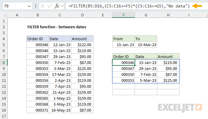
This is another example of using multiple criteria: the first expression checks that each date is on or after the start date, the second checks that it is on or before the end date, and multiplication (*) requires both to be TRUE with AND logic. The matching orders spill into the range F8:H11.

For more details, see Filter data between dates.

When no records meet supplied conditions, FILTER will return a #CALC! error. In the formula above, notice the third argument, if_empty, is set to "No data" so the formula shows a friendly message instead of a #CALC! error when no orders fall in the range. You can also supply an empty string ("") to display nothing when no data is returned.

Filter where text contains

FILTER does not support wildcards directly, but you can filter for values that contain specific text by pairing FILTER with the SEARCH and ISNUMBER functions. In the worksheet below, the goal is to extract addresses that contain "rd". The formula in cell D5 is:

=FILTER(B5:B16,ISNUMBER(SEARCH("rd",B5:B16)),"No results")

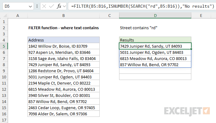
Working from the inside out: SEARCH looks for "rd" in each address and returns the position of the match as a number, or a #VALUE! error when there is no match. ISNUMBER then converts those results into TRUE (found) and FALSE (not found), which becomes the include argument. Because SEARCH is not case-sensitive, it matches "rd" in "Rd" as well. The matching addresses spill into the range D5:D8, and if_empty returns "No results" when nothing matches.

Note that SEARCH itself supports Excel's wildcards (* and ?), so you can build more flexible "contains" logic when you need it. For a full explanation, see Filter where text contains.

If you need to filter based on sophisticated pattern matching, combine FILTER with the new REGEXTEST function which lets you use Regular Expressions in your formulas.

Filter top N values

You can combine FILTER with the LARGE function to extract the top N records by value. In the worksheet below, the goal is to extract the rows with the top 3 scores. The formula in cell F5 is:

=FILTER(B5:D16,D5:D16>=LARGE(D5:D16,3))

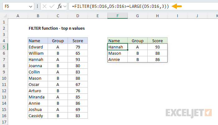
LARGE(D5:D16,3) returns the 3rd largest score, which acts as a threshold. The logical expression D5:D16>=LARGE(D5:D16,3) then returns TRUE for any score at or above that threshold, and FILTER returns the matching rows. To get a different number of records, change the second argument to LARGE: use 5 for the top 5, 10 for the top 10, and so on. The three top-scoring records spill into the range F5:H7.

Keep in mind that ties can return more rows than expected. If two records share the Nth value, both are included. For more details, see Filter top n values.

Filter and sort

Because FILTER returns a dynamic array, you can wrap it in other dynamic array functions like SORT. In the worksheet below, the goal is to extract orders on or after March 1, 2026, sorted by amount from largest to smallest. The formula in cell F5 is:

=SORT(FILTER(B5:D16,C5:C16>=DATE(2026,3,1)),3,-1)

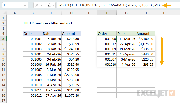
FILTER runs first and extracts the orders that meet the date condition, using the DATE function to build the cutoff date. SORT then reorders that result: the second argument (3) sorts by the third column (Amount), and the third argument (-1) sorts in descending order. The final result spills into the range F5:H10. Nesting dynamic array functions like this is a clean way to shape output without helper columns.

For more details, see Filter and sort without errors.

Filter horizontal data

FILTER works with horizontal data as well as vertical data. When the data is arranged in columns, you filter columns instead of rows by supplying a horizontal include array. In the worksheet below, the data runs across rows 4 to 6, and the goal is to return only the people whose Age is less than 22. The formula in cell C9 is:

=FILTER(C4:L6,C6:L6<22)

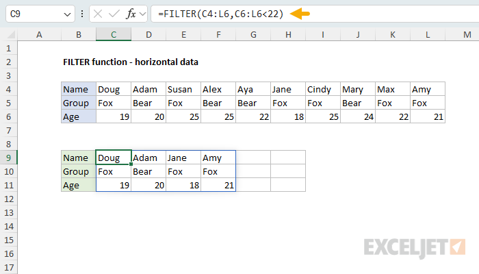
The array is the horizontal block C4:L6, and the include argument is the single row C6:L6, which holds the ages. The expression C6:L6<22 returns a horizontal array of TRUE and FALSE values, one per column, and FILTER keeps the columns where the result is TRUE. Notice that the include array is horizontal to match the orientation of the data: when you filter columns, include must be a single row; when you filter rows, it must be a single column. The four matching columns spill into the range C9:F11.

For more details, see Filter horizontal data.

Complex multiple criteria

The Boolean logic approach scales to as many conditions as you need. In the worksheet below, the goal is to extract records that meet three separate conditions at once: the Account begins with "x", AND the Region is "east", AND the month is NOT April. The formula in cell G5 is:

=FILTER(B5:E16,(LEFT(B5:B16)="x")*(C5:C16="east")*NOT(MONTH(D5:D16)=4))

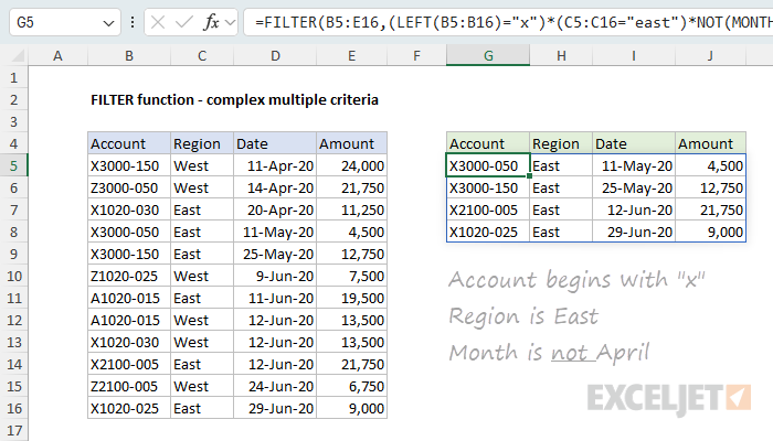
Each condition is its own logical expression. The LEFT function checks whether the account begins with the letter "x", and the NOT and MONTH functions are used to exclude transactions in April. The include argument, with line breaks added for readability, looks like this:

(LEFT(B5:B16)="x")*    // begins with "x"
(C5:C16="east")*       // region is East
NOT(MONTH(D5:D16)=4)   // not April

Multiplying the three expressions together applies AND logic, so a record must meet all three conditions to be included. The matching records spill into the range G5:J8. Building criteria this way is an elegant and flexible approach that can be extended to handle many complex scenarios.

For more details, see Filter with complex multiple criteria.

Notes

• FILTER is available in Excel 2021+ and Excel 365. It is not available in earlier versions of Excel.
• The include argument must have dimensions compatible with the array argument, or FILTER will return a #VALUE! error. When filtering rows, include is a single column; when filtering columns, it is a single row.
• If FILTER finds no matching data and no if_empty argument is provided, it returns a #CALC! error. Supply if_empty to return a message or an empty string ("") instead.
• If the include array contains an error, FILTER will return that error.
• Results spill onto the worksheet. If a cell in the spill range is not empty, FILTER returns a #SPILL! error; clear the blocking cells to resolve it.
• FILTER preserves the original order of the source data. Wrap FILTER in SORT to reorder the results.
• To remove duplicate rows from a filtered result, wrap FILTER in the UNIQUE function.
• FILTER can work with both vertical and horizontal arrays.