Summary
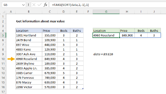
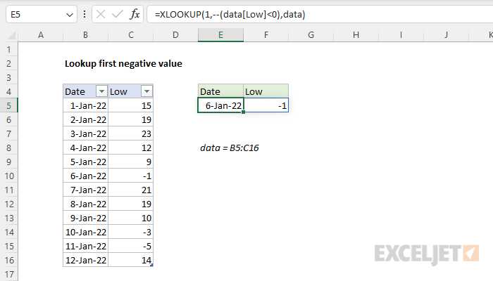
To lookup the first negative value in a set of data, you can use the XLOOKUP function. In the example shown, the formula in cell E5 is:
=XLOOKUP(1,--(data[Low]<0),data)
where data is an Excel Table in the range B5:C16. The result is the sixth row in the table, since this is the first negative value in the Low column. Because we provide data for return_array, the result includes both the date and the value. See below for details and alternatives.
Generic formula
=XLOOKUP(1,--(range<0),range)
Explanation
In this example, the goal is to lookup the first negative value in a set of data. In addition, we also want to get the corresponding date. All data is in an Excel Table called data, in the range B5:C16. This information represents the low temperature in Fahrenheit (F) for the dates as shown. There are several ways to solve this problem, as explained below.
XLOOKUP function
A simple solution is to use the XLOOKUP function with Boolean logic. This is the approach in the workbook shown, where the formula in cell E5 is:
=XLOOKUP(1,--(data[Low]<0),data)
Notice that lookup_value is given as 1. In this particular example, we could use TRUE instead of 1. However, you will often see 1 used as a lookup value because it is compact, and because it will continue to work nicely as the logic to target specific values becomes more complex.
To target negative values, lookup_array is provided as this expression:
--(data[Low]<0)
Since there are 12 values in data[Low], the result inside the parentheses is an array of 12 TRUE and FALSE values like this:
{FALSE;FALSE;FALSE;FALSE;FALSE;TRUE;FALSE;FALSE;FALSE;TRUE;TRUE;FALSE}
Because we have already set lookup_value to 1, we need to convert this array to the numeric values 1 and 0. The double negative (--) is a simple way to perform this conversion. The resulting array looks like this:
{0;0;0;0;0;1;0;0;0;1;1;0}
The 1s in this array correspond to the negative numbers in the Low column. The array is returned directly to XLOOKUP as the lookup_array, so we can rewrite the formula at this point like this:
=XLOOKUP(1,{0;0;0;0;0;1;0;0;0;1;1;0},data)
By default, XLOOKUP will match the first occurrence of the lookup_value, so it matches the 1 at row 6. Because the return_array is given as data, (B5:C16) XLOOKUP returns row 6 from the table as a final result. The two values in row 6 spill into cells E5 and F5 as shown.
As an alternative to the single formula above, you could use two separate formulas like this:
=XLOOKUP(1,--(data[Low]<0),data[Date]) // date
=XLOOKUP(1,--(data[Low]<0),data[Low]) // low
Notice the only difference in these formulas is the value given for the result_array.
INDEX and MATCH
This problem can also be solved with an INDEX and MATCH formula like this:
=INDEX(data,MATCH(1,--(data[Low]<0),0),0)
Notice that the MATCH function is configured like the XLOOKUP function above. Also note that column_num inside INDEX is given as 0, to cause the INDEX function to return an entire row of data (i.e. both Date and Low). After the expression data[Low]<0 is evaluated and converted to 1s and 0s, we have:
=INDEX(data,MATCH(1,{0;0;0;0;0;1;0;0;0;1;1;0},0),0)
Next, MATCH returns the position of the first 1 in lookup_array (6) to INDEX as row_num:
=INDEX(data,6,0)
Finally, INDEX returns row 6 from data as a final result. As with XLOOKUP above, you could also use two separate formulas like this:
=INDEX(data,MATCH(1,--(data[Low]<0),0),1) // date
=INDEX(data,MATCH(1,--(data[Low]<0),0),2) // low
Notice the only difference is the value provided for column_num.
Note: this is an array formula that must be entered with Control + Shift + Enter in Legacy Excel.
FILTER function
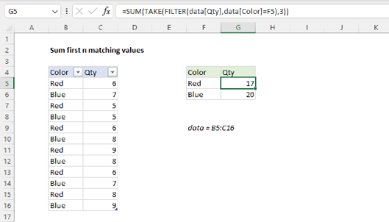
Another interesting way to solve this problem is to use the FILTER function with the TAKE function, like this:
=TAKE(FILTER(data,data[Low]<0),1)
Working from the inside out, FILTER is given data for array, and the expression data[Low]<0 for the include argument. With this configuration, FILTER returns the 3 rows in data that have negative values in the Low column. Note that the result from FILTER includes both columns, Date and Low. This data is returned directly to the TAKE function as the array argument, with row given as 1. TAKE then returns just row 1 from the matching data as a final result.
TAKE is a new function. If you have a version of Excel without take, you can use INDEX instead, like this:
=INDEX(FILTER(data,data[Low]<0),1)
Note: Without the TAKE or INDEX, FILTER will return and display all 3 rows in data that have negative values in the Low column.