=IF(logical_test, [value_if_true], [value_if_false])- logical_test - A value or logical expression that can be evaluated as TRUE or FALSE.
- value_if_true - [optional] The value to return when logical_test evaluates to TRUE.
- value_if_false - [optional] The value to return when logical_test evaluates to FALSE.
Using the IF function
The IF function is one of the most widely used functions in Excel. At the core, IF runs a test and returns one value when the result is TRUE, and another value when the result is FALSE. At first glance, this seems very basic — if this is true, do this; otherwise, do that. However, formulas that use IF can quickly become advanced as the requirements become more complex and more IFs are nested together. One of the tricks in using IF effectively is knowing how to combine IF with other functions like AND and OR to handle more complex logic gracefully. This article explains the basics carefully, then introduces more advanced formulas that use the IF function.
Key features
- Performs logical tests that return TRUE or FALSE
- Returns different results based on whether the test is TRUE or FALSE
- Works with all comparison operators (=, <>, >, <, >=, <=)
- Both value_if_true and value_if_false are optional, but at least one must be provided
- Can be combined with AND, OR, and NOT for complex logical tests
- Supports nested IF statements for multiple conditions ("else if" logic)
- Not case sensitive and does not support wildcards directly
- Can be combined with SEARCH and ISNUMBER for simple pattern matching
- Can be combined with REGEXTEST for advanced pattern matching
- Can return empty strings ("") to make cells appear blank
- Works in all versions of Excel
The IF function can be deceptively simple. Many Excel users have gotten into the weeds debugging a complicated nested IF formula that doesn't even make sense for the problem at hand. If an IF formula seems too long and complicated, there is almost certainly a better way to do it in Excel. To avoid this fate, it pays to understand the basics well and know when to seek other solutions.
Contents
- Basic IF function example
- Logical tests
- Example - Pass or Fail
- Example - IF this OR that
- Example - IF this AND that
- Example - IF this AND OR that
- Example - Nested IF
- Example - Return another formula with IF
- Example - IF contains specific text
- Example - IF with wildcards and regex
- When not to use IF
Basic IF function example
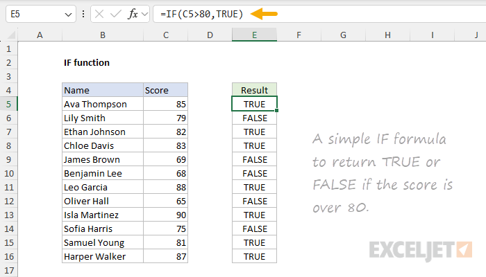
To understand how the IF function works, let's start with a very basic example. In the worksheet below, the goal is to use the IF function to mark scores greater than 80 with an IF formula. The simplest IF we can write for this looks like this:
=IF(B5>80,TRUE)
Translation: If B5 is greater than 80, return TRUE. You can see the result in the worksheet below.
Note we are not using quotes ("") anywhere in the formula because the formula contains no text. Also, we do not need to provide a value for value_if_false because IF will return FALSE by default. This formula works fine. But the output is rather busy and hard to read. Let's change the formula to return an "x" when the score is over 80:
=IF(B5>80,"x")
Notice that the "x" appears in double quotes because it is a text value. Text values hardcoded into formulas must always be quoted. You can see the result below:
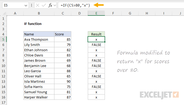
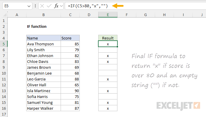
Note that TRUE values have been replaced by "x", and the FALSE results remain FALSE since we have not provided a value for value_if_false. Finally, let's modify the formula to display nothing when a score is not over 80. We can do this by providing an empty string ("") for value_if_false like this:
=IF(B5>80,"x","")
After updating the formulas in column E, the output is much easier to read. We now see an "x" for scores over 80. For scores that are not over 80, the cells appear to be empty:
Remember: text values like "x" must be enclosed in double-quotes. Numbers like 80 are not quoted.
Logical tests
Before we move on, let's talk more about how logical tests work in the IF function. Usually, the logical_test in IF is an expression that will return TRUE or FALSE. The table below shows some common examples:
| Goal | Logical test |
|---|---|
| If A1 is greater than 75 | A1>75 |
| If A1 equals 100 | A1=100 |
| If A1 is less than or equal to 100 | A1<=100 |
| If A1 equals "Red" | A1="red" |
| If A1 is not equal to "Red" | A1<>"red" |
| If A1 is less than B1 | A1<B1 |
| If A1 is empty | A1="" |
| If A1 is not empty | A1<>"" |
| If A1 is less than the current date | A1<TODAY() |
Notice that text values that appear in a logical test must be enclosed in quotes (""). However, numbers and logical operators like >,<,<>,=, etc., are not quoted.
Note: The IF function is not case-sensitive. The text "red" will match "red", "Red", "RED", or "rEd".
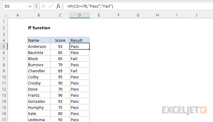
Example - Pass or Fail
In the worksheet below, we want to assign either a "Pass" or "Fail" based on a test score. A passing score is 70 or higher. The formula in E5, copied down, is:
=IF(C5<70,"Fail","Pass")
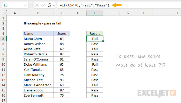
Notice both "Pass" and "Fail" are in double quotes ("") because they are text values. Also, note that the logical flow of this formula can be reversed. Above, we test for failing scores. To test for passing scores, we can write a formula like this:
=IF(C5>=70,"Pass","Fail")
Translation: If the value in C5 is greater than or equal to 70, return "Pass". Otherwise, return "Fail". Both formulas will return the same result. Which option you choose is a personal preference.
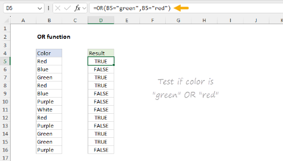
Example - IF this OR that
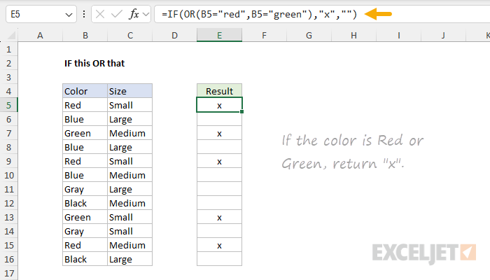
A common challenge with the IF function is how to handle a problem that requires "if this or that" logic. The logical test for IF takes just one value, so how do you test for more than one result? The trick is to combine the IF function with the OR function. For example, the goal in the worksheet below is to mark rows where the color is "Red" OR "Green". We can write a formula that does this by combining the IF function with the OR function like this:
=IF(OR(B5="red",B5="green"),"x","")
Translation: If the value in B5 is "red" or "green", return "x". Otherwise, return an empty string ("").
Notice that the OR function is embedded inside the IF function as the logical test. The OR function accepts multiple logical expressions. If any expression returns TRUE, the OR function will return TRUE. Only if all logical expressions return FALSE will the OR function return FALSE. You can see the result below:
Video: IF this OR that
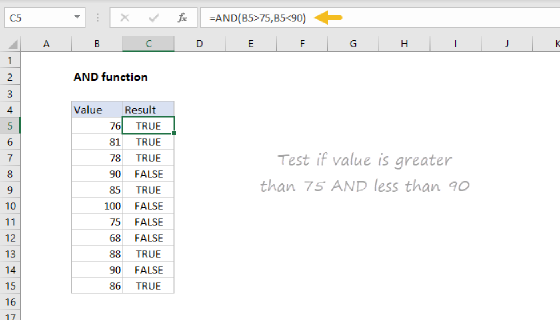
Example - IF this AND that
Like the OR function, the AND function can be combined with the IF function to create "if this AND that logic". In the worksheet below, the goal is to mark people in group B with a score of at least 80. The formula in cell F5, copied down, is:
=IF(AND(C5="B",D5>=80),"x","")
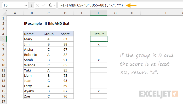
Notice the AND function is nested in the IF function as the logical test and contains two logical expressions: C5="B", and D5>=80. The "B" appears in quotes ("") because it is a text string. The 80 is not quoted because it is a number.
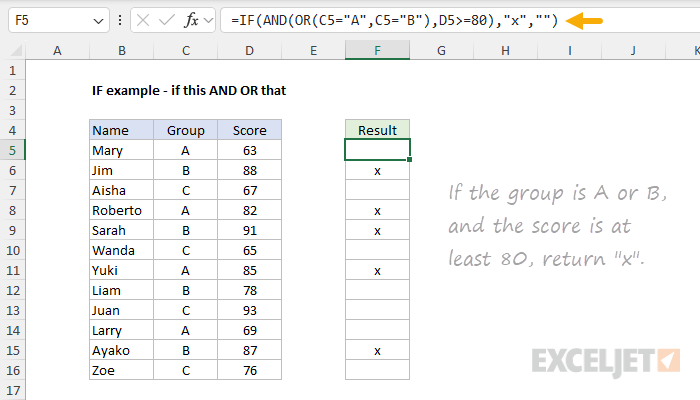
Example - IF this AND OR that
You can combine the AND and OR functions inside IF to implement more advanced logic. In the example below, the goal is to mark people in groups A or B with a score of at least 80. The formula in cell F5, copied down, is:
=IF(AND(OR(C5="A",C5="B"),D5>=80),"x","")
Example - Nested IF
The IF function can be "nested". A "nested IF" refers to a formula where one IF function is nested inside another to test for more conditions and return more possible results. Each IF statement needs to be carefully "nested" inside another so that the logic is correct. The idea here is that we are chaining together multiple IF functions to create "else if" logic. In the example below, the goal is to assign a number to each color. If the color is Red, the result should be 100. If the color is Blue, the result should be 125. If the color is Green, the result should be 150. In the worksheet below, the formula in D5 is a "nested IF" like this:
=IF(B5="red",100,IF(B5="blue",125,IF(B5="green",150)))
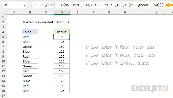
Translation: If the color is Red, 100, else if the color is Blue, 125, else if the color is Green, 150.
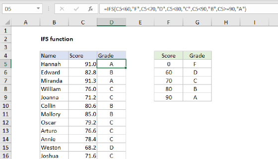
Note that this formula will only handle three colors: Red, Blue, and Green". With any other color, the formula will return FALSE. As you might expect, you can add more IF functions to handle more values. See this page for a more advanced nested IF to assign grades. However, before you go down that road, be aware that Excel has other options to handle multiple tests. For example, the IFS function can handle multiple logical tests without nesting with a formula like this:
=IFS(B5="red",100,B5="blue",125,B5="green",150)
You can also use the SWITCH function with an even simpler formula like this:
=SWITCH(B5,"red",100,"blue",125,"green",150)
Both formulas above will return the same result as the original nested IF formula.
Note: For more complex scenarios with many values to test, consider other functions, like VLOOKUP or XLOOKUP, because they can handle more conditions in a more streamlined fashion.
Example - Return another formula with IF
As seen above, the IF function can easily return another value when the result of a test is TRUE or FALSE. In addition, the IF function can also return a formula. For example, in the worksheet below, the goal is to increase the price of Red items only by 20%. The price of other colors should remain unchanged. The formula in cell F5 is:
=IF(B5="red",D5*1.2,D5)
As the formula is copied down, it tests the color in column B. If the color is Red, it returns D5*1.2, effectively increasing the price by 20%. If the color is not Red, it simply returns D5. You can see the result below:
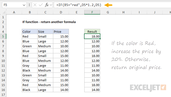
Notice the results in column F. Most prices are the same, but prices for the color Red are now 20% higher. Although this is a simple formula, IF can return any normal Excel formula for both TRUE and FALSE results.
Example - IF contains specific text
Because the IF function does not support wildcards directly, it is not obvious how to configure IF to check for a specific substring in a cell. A common approach is to combine the ISNUMBER function and the SEARCH function to create a logical test like this:
=ISNUMBER(SEARCH(substring,A1)) // returns TRUE or FALSE
For example, to check for the substring "xyz" in cell A1, you can use a formula like this:
=IF(ISNUMBER(SEARCH("xyz",A1)),"Yes","No")
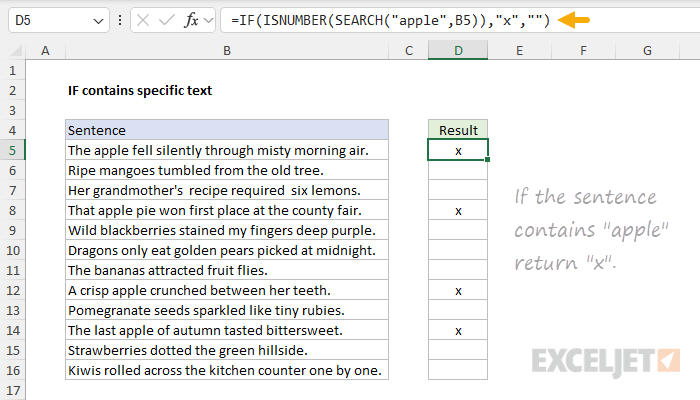
In the worksheet below, we want to test each sentence in column B for the word "apple". The formula in cell D5, copied down, is:
=IF(ISNUMBER(SEARCH("apple",B5)),"x","")
Because the SEARCH function supports basic Excel wildcards, you can include these in your IF formula. Read a more detailed explanation here.
IF with wildcards and regex
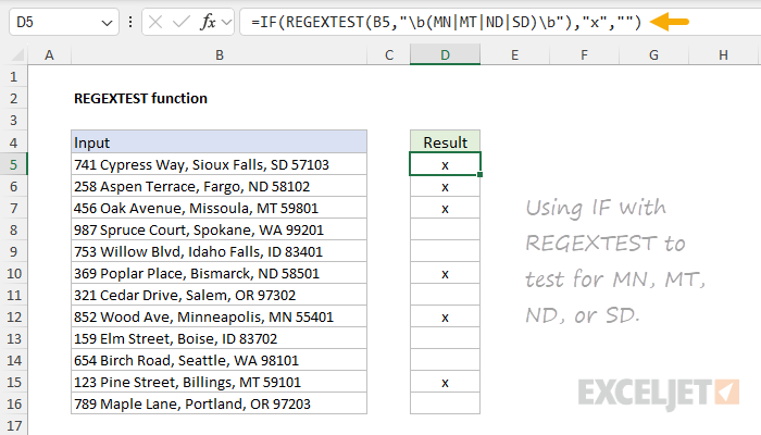
The IF function does not support wildcards directly. However, you can combine IF with other Excel functions to overcome this limitation. For basic wildcard support, you can combine IF with COUNTIF or combine IF with SEARCH (as seen above). If you need more than basic wildcards, you can use the full power of Regular Expressions by combining IF with the REGEXTEST function. REGEXTEST tests for a regex pattern and returns TRUE or FALSE, making it a perfect fit for the IF function. For example, in the worksheet below, the goal is to test the input in column B for four US states based on their two-letter abbreviations: MN, MT, ND, and SD. This can be done with the pattern ""\b(MN|MT|ND|SD)\b". The formula in D5, copied down, is:
=IF(REGEXTEST(B5,"\b(MN|MT|ND|SD)\b"),"x","")
For more information on regex in Excel, see: Regular Expressions in Excel.
When not to use IF (related functions)
IF is a widely used function in Excel, and you'll find it in all kinds of worksheets in almost any industry. However, just because IF is common doesn't mean you should always use it. Excel has many functions that can apply conditional logic. Here are some good options, depending on your specific use case:
- IFS function - Handles multiple conditions without nesting
- SWITCH function - Match a single value against multiple options
- CHOOSE function - Return values based on position/index numbers
- XLOOKUP / VLOOKUP - Better than nested IFs for matching values in tables
- COUNTIFS / SUMIFS - Apply conditional logic for counting/summing without IF
- FILTER function - Extract matching records based on matching criteria
Before you try to make IF do something it's not well suited for, make sure you have an idea of what Excel offers out of the box. See 101 Functions You Should Know, Dynamic Array Formulas in Excel, and New Excel Functions for more information.
Notes
- The IF function is not case-sensitive.
- Inside IF, text values should be enclosed in double quotes ("").
- Numbers and logical values like TRUE and FALSE should not be quoted.
- IF does not support wildcards, but can be combined with other functions that do.
- To extract records that meet specific criteria, see the FILTER function.
- To count values that meet specific criteria, use the COUNTIF or the COUNTIFS functions.
- To sum values that meet specific criteria, use the SUMIF or the SUMIFS functions.