Summary
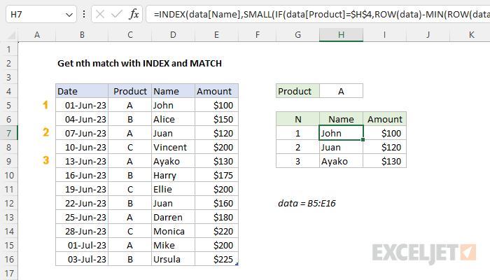
To get the nth matching record in a set of data with an INDEX and MATCH formula, you can use a formula like this in cell H7:
=INDEX(data[Name],SMALL(IF(data[Product]=$H$4,ROW(data)-MIN(ROW(data))+1),G7))
Where data is an Excel Table in the range B5:E16. When H4 contains "A", the formula will return the 1st, 2nd, and 3rd names that correspond with product "A" in the table. A similar formula can be used to return the Amount in cell I7. See below for details. Note this is an array formula that must be entered with control + shift + enter in Excel 2019 and earlier.
Note: The purpose of this example is to explain how to get the nth match in Excel 2019 and older with an INDEX and MATCH formula. In the current version of Excel, the FILTER function is a much better way to get multiple matching records.
Generic formula
=INDEX(rng,SMALL(IF(rng=A1,ROW(rng)-MIN(ROW(rng))+1),n))
Explanation
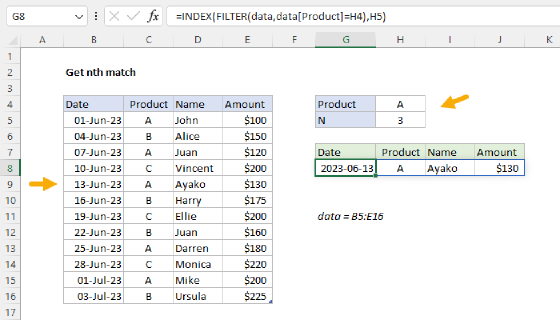
The goal is to retrieve the nth matching record in a table when targeting a specific product. For example, if the value in cell H4 is "A", the formula in H7 should return the name "John", since this is the first name in the table associated with product "A". In the same way, the formula in H8 should return 'Juan', since this is the second name associated with product "A". The product in H4 is an input that can be changed at any time. All data exists in an Excel Table named data.
Basic INDEX and MATCH
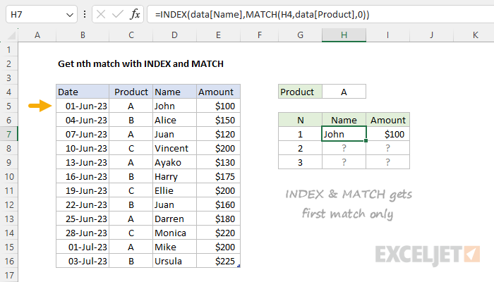
Before we look at the formula used in the worksheet, we should review why we can't use a "normal" INDEX and MATCH formula to solve this problem. Normally, the INDEX and MATCH functions are used to find the position of a value in a table and return a corresponding value in the same position from a different column. However, this method only works for the first match. For example, in the screen below, these the INDEX and MATCH formulas in H7 and I7 are as follows:
=INDEX(data[Name],MATCH(H4,data[Product],0)) // returns "John"
=INDEX(data[Amount],MATCH(H4,data[Product],0)) // returns 100
In these formulas, the MATCH function is configured to match the value in H4 ("A"), in the Product column. In both formulas, MATCH returns 1 because the product is "A". These formulas work perfectly, but the problem is that we have no way to ask MATCH to find the 2nd match, the 3rd match, etc.
As mentioned, this is a standard application of INDEX and MATCH. For a complete overview, see: How to use INDEX and MATCH.
INDEX and SMALL + IF
One workaround to the INDEX and MATCH limitation explained above is to use INDEX with the SMALL and IF instead of MATCH. At the core, this approach uses INDEX to get the name at a specific row number like this:
=INDEX(data[Name],row_num)
The challenge is how to calculate the row number for each nth match since MATCH will only find the first match. One workaround is to generate a set of row numbers for the entire table, then use the IF function to "filter" the row numbers based on the product specified in cell H4. Then we can give this filtered list to the SMALL function, which is designed to get the "nth smallest" value. That is the approach seen in the worksheet as shown, where the formula in H7 is as follows:
=INDEX(data[Name],SMALL(IF(data[Product]=$H$4,ROW(data)-MIN(ROW(data))+1),G7))
Note this is an array formula that must be entered with control + shift + enter in Excel 2019 and earlier.
All of the hard work in this formula is in determining a row number for INDEX, which is done here:
SMALL(IF(data[Product]=$H$4,ROW(data)-MIN(ROW(data))+1),G7)
This may look complicated, but the approach is pretty straightforward. We create row numbers for the data, filter the numbers with an appropriate logical test, then retrieve the nth matching row number. Working from the inside out, the code below generates a set of relative row numbers for the entire table:
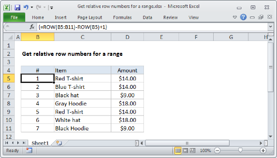
ROW(data)-MIN(ROW(data))+1
Since there are 12 rows in the table, the result is an array like this:
{1;2;3;4;5;6;7;8;9;10;11;12}
For more details on how this works, see this page. Simplifying the formula, we now have:
SMALL(IF(data[Product]=$H$4,{1;2;3;4;5;6;7;8;9;10;11;12}),G7)
Next, the IF function applies a logical test to filter on numbers where the product is "A" in H4:
IF(data[Product]=$H$4,{1;2;3;4;5;6;7;8;9;10;11;12})
Because there are 12 rows in the table, the result is an array like this:
{1;FALSE;3;FALSE;5;FALSE;FALSE;FALSE;9;FALSE;11;FALSE}
Notice the only numbers to survive the filtering are the rows associated with product "A". The other row numbers have been replaced by FALSE. Next, the SMALL function is used to return the nth smallest value:
SMALL({1;FALSE;3;FALSE;5;FALSE;FALSE;FALSE;9;FALSE;11;FALSE},G7)
SMALL automatically ignores the FALSE values. With 1 in cell G7, SMALL returns the smallest value, which is 1. This is returned directly to the INDEX function as row_num. Back in the original formula, we now have:
=INDEX(data[Name],1) // returns "John"
The INDEX function then returns "John" in cell H7. In cell H8, the value in G8 is 2, and SMALL returns the second smallest row number, which is 3:
=INDEX(data[Name],3) // returns "Juan"
As the formula is copied down, the value for n increases in column G causing the SMALL function to retrieve the next matching row number. At each new row, the formula returns the next nth match.
Retrieving Amount
The formula to retrieve the associated Amount is almost exactly the same as the formula above:
=INDEX(data[Amount],SMALL(IF(data[Product]=$H$4,ROW(data)-MIN(ROW(data))+1),G7))
The only difference is the value for the array provided to INDEX, which is data[Amount] instead of data[Name].
Handling errors
Once there are no more matches for a given value of n, the SMALL function will return a #NUM error. You can handle this error with the IFERROR function, or by adding logic to count matches and abort processing once the number in column H is greater than the match count. The example here shows one approach.
Multiple criteria
To add multiple criteria, you use boolean logic, as explained in this example.