Summary
To lookup values with INDEX and MATCH, using multiple criteria, you can use an array formula. In the example shown, the formula in H8 is:
=INDEX(E5:E11,MATCH(1,(H5=B5:B11)*(H6=C5:C11)*(H7=D5:D11),0))
The result is $17.00, the price of a Large Red T-shirt. This is an array formula and must be entered with Control + Shift + Enter in Legacy Excel.
Note: In the current version of Excel, you can use the same approach with the XLOOKUP function.
Generic formula
=INDEX(range1,MATCH(1,(A1=range2)*(B1=range3)*(C1=range4),0))
Explanation
This is a more advanced formula. For basics, see How to use INDEX and MATCH.
Normally, an INDEX MATCH formula is configured with MATCH set to look through a one-column range and provide a match based on given criteria. Without concatenating values in a helper column, or in the formula itself, there's no way to supply more than one criteria.
This formula works around this limitation by using boolean logic to create an array of ones and zeros to represent rows matching all 3 criteria, then using MATCH to match the first 1 found. The temporary array of ones and zeros is generated with this snippet:
(H5=B5:B11)*(H6=C5:C11)*(H7=D5:D11)
Here we compare the item in H5 against all items, the size in H6 against all sizes, and the color in H7 against all colors. The initial result is three arrays of TRUE/FALSE results like this:
{TRUE;TRUE;TRUE;FALSE;FALSE;FALSE;TRUE}*{FALSE;FALSE;TRUE;FALSE;FALSE;TRUE;FALSE}*{TRUE;FALSE;TRUE;FALSE;FALSE;FALSE;TRUE}
Tip: use F9 to see these results. Just select an expression in the formula bar, and press F9.
The math operation (multiplication) transforms the TRUE FALSE values to 1s and 0s:
{1;1;1;0;0;0;1}*{0;0;1;0;0;1;0}*{1;0;1;0;0;0;1}
After multiplication, we have a single array like this:
{0;0;1;0;0;0;0}
which is fed into the MATCH function as the lookup array, with a lookup value of 1:
MATCH(1,{0;0;1;0;0;0;0})
At this point, the formula is a standard INDEX MATCH formula. The MATCH function returns 3 to INDEX:
=INDEX(E5:E11,3)
and INDEX returns a final result of $17.00.
Array visualization
The arrays explained above can be difficult to visualize. The image below shows the basic idea. Columns B, C, and D correspond to the data in the example. Column F is created by multiplying the three columns together. It is the array handed off to MATCH.

Non-array version
It is possible to add another INDEX to this formula, avoiding the need to enter as an array formula with control + shift + enter:
=INDEX(rng1,MATCH(1,INDEX((A1=rng2)*(B1=rng3)*(C1=rng4),0,1),0))
The INDEX function can handle arrays natively, so the second INDEX is added only to "catch" the array created with the boolean logic operation and return the same array again to MATCH. To do this, INDEX is configured with zero rows and one column. The zero row trick causes INDEX to return column 1 from the array (which is already one column anyway).
Why would you want the non-array version? Sometimes, people forget to enter an array formula with control + shift + enter, and the formula returns an incorrect result. So, a non-array formula is more "bulletproof". However, the tradeoff is a more complex formula.
Note: In Excel 365, it is not necessary to enter array formulas in a special way.