Summary
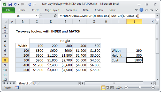
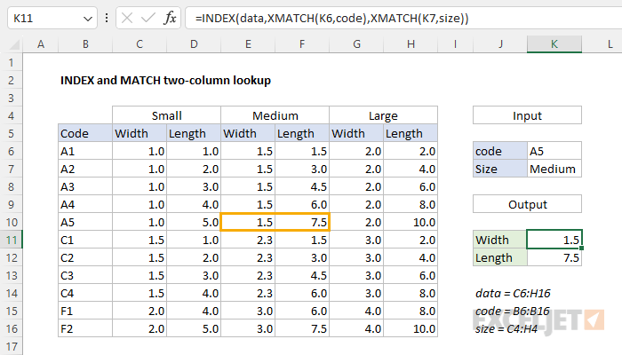
To create a lookup formula that returns two columns from the source data, you can use an INDEX and MATCH formula. In the example shown, the formulas in K11 and K12 are, respectively:
=INDEX(data,XMATCH(K6,code),XMATCH(K7,size)) // width
=INDEX(data,XMATCH(K6,code),XMATCH(K7,size)+1) // height
Where data (C6:H16), code (B6:B16), and size (C4:H4) are named ranges. With "A5" in cell K6, and "Medium" in cell K7, the first formula returns a Width of 1.5 and the second formula returns a Length of 7.5. When the inputs for code (K6) or size (K7) are changed, the formulas calculate a new result.
Notes: (1) the values in row 4 are not merged cells but instead use "Center across selection" alignment as explained below. (2) It is possible to use the XLOOKUP function as well. See below for details.
Generic formula
=INDEX(data,XMATCH(A1,array),XMATCH(array,array))
Explanation
In this example, the goal is to look up Width and Length based on inputs for Code (K6) and Size (K7). While finding the correct row based on the Code value is straightforward, the problem of how to best retrieve both columns of data (Width and Length) is more challenging. One good way to solve this problem is with an INDEX and MATCH formula, but you can also use XLOOKUP as explained below. For convenience, data (C6:H16), code (B6:B16), and size (C4:H4) are named ranges.
Note: If you are new to INDEX with MATCH, see this overview: How to use INDEX and MATCH.
Heading configuration
One important detail in this problem is that the Size information in row 4 is configured in a special way. The values "Small", "Medium", and "Large" appear in cells C1, E1, and G1, respectively. The cells in row 4 are not merged. To show each Size centered over the two columns for Width and Length, the Horizontal Alignment is set to Center Across Selection as seen below:
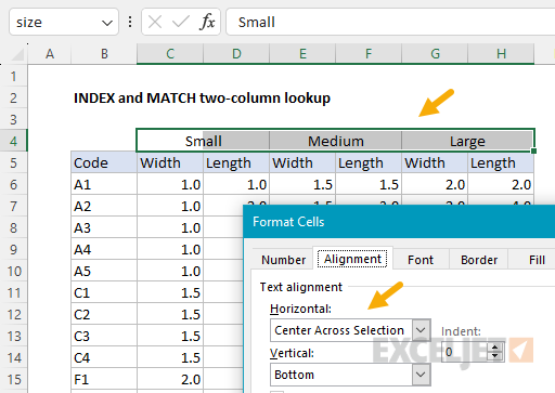
This is important because we need to match the correct size, which must correspond to the six columns of data. In other words, when we match "Medium", we need to get a reference to column 3, as explained in more detail below. Note that this means some cells in row 4 are blank, but this doesn't matter as long as we use an exact match setting for MATCH or XMATCH.
Two-way INDEX and MATCH
Essentially, this formula uses a standard two-way INDEX and MATCH formula. The INDEX function is provided with the data to return, and the MATCH function is used two times. The first MATCH calculates the correct row number, and the second MATCH calculates the correct column number(s). The generic syntax looks like this:
=INDEX(data,XMATCH(),XMATCH())
Note: We are using XMATCH in this example because the configuration is slightly simpler since XMATCH defaults to an exact match, so there is no need to provide match_type. However, the regular MATCH function will work fine as well.
In the worksheet shown, the specific formula used in cell K11 is:
=INDEX(data,XMATCH(K6,code),XMATCH(K7,size))
Working from the inside out, the first XMATCH function returns a row based on the code in cell K6:
XMATCH(K6,code) // returns 5
Because "A5" is the fifth value in code (B6:B16), the first XMATCH function returns 5. The second XMATCH function is used to find the correct column, like this:
XMATCH(K7,size) // returns 3
Because "Medium" is the third value in size (C4:H4), the MATCH function returns 3. After simplifying the formula to show the results returned by XMATCH, we have the following:
=INDEX(data,5,3) // returns 1.5
INDEX then retrieves the value at row 5 and column 3 in data (C6:H16), which is 1.5. The formula to return the Length in cell K12 is almost exactly the same:
=INDEX(data,XMATCH(K6,code),XMATCH(K7,size)+1)
Notice the only difference is that we are adding 1 to the column number. The result is that we retrieve the value in the next column, which holds the value for Length. The formula works like this:
=INDEX(data,5,3+1)
=INDEX(data,5,4)
=7.5
With the MATCH function
As mentioned above, you can use the regular MATCH function instead of XMATCH, but you must provide 0 for match_type to enable an exact match like this:
=INDEX(data,MATCH(K6,code,0),MATCH(K7,size,0))
=INDEX(data,MATCH(K6,code,0),MATCH(K7,size,0)+1)
For more details, see How to use the MATCH function.
Single formula
You can modify the formula slightly to return both Width and Length at the same time:
=INDEX(data,XMATCH(K6,code),XMATCH(K7,size)+{0;1})
Notice the only change is to replace 1 with the array constant {0;1}. The formula now evaluates like this:
=INDEX(data,5,3+{0;1})
=INDEX(data,5,{3;4})
={1.5;7.5}
By adding 0 and 1 to the column number returned by XMATCH, we end up with two numbers in an array {3;4} that are provided to the INDEX function as column_num. The result is that INDEX returns values from both columns, and these values spill into the range K11:K12 when using a current version of Excel.
You might notice that we provided the array constant as {0;1} and not {1,0}. By providing the values in rows, we get back a vertical array. If we used {1,0} instead, we would get a horizontal array and would need to use the TRANSPOSE function to flip the orientation of the final result.
XLOOKUP
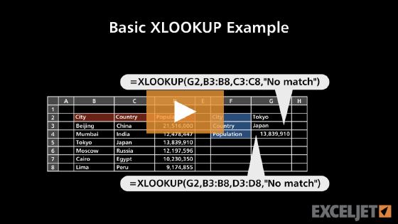
This problem can also be solved with the XLOOKUP function, but the formula is not quite as straightforward. We start by configuring XLOOKUP to match the code like this:
=XLOOKUP(K6,code,data)
This formula will return the entire row of widths and lengths for the code entered in K6. Next, we can nest this formula inside a second XLOOKUP, which has been configured to retrieve the size:
=XLOOKUP(K7,size,XLOOKUP(K6,code,data))
The inner XLOOKUP retrieves all the values for "A5" in an array, and the outer XLOOKUP selects the correct value for Width based on a size of "Medium" (1.5). However, getting the Length is more challenging because we can't just add 1 as we did with INDEX and MATCH above. Instead of nesting one XLOOKUP inside another, I think a better approach is to use the XLOOKUP together with XMATCH and the newer CHOOSECOLS function like this:
=CHOOSECOLS(XLOOKUP(K6,code,data),XMATCH(K7,size)) // width
=CHOOSECOLS(XLOOKUP(K6,code,data),XMATCH(K7,size)+1) // length
As before, the inner XLOOKUP retrieves all the values for the code in K6 in an array. This time, however, the array is returned to the CHOOSECOLS function, which uses XMATCH to select the Width based on the size in K7. As in the original example above, XMATCH matches on size and returns a column number. CHOOSECOLS then returns the specified column. Because CHOOSECOLS uses a numeric index for a column, we can simply add 1 to the first formula to get Length, just as we did in the INDEX and MATCH formula above.
This works fine, and it's a nice demonstration of how CHOOSECOLS can make it possible to use a numeric index for columns. However, we now have three functions in the mix, and I don't see any advantage to using XLOOKUP in this case. Let me know if you disagree!
Note: because XLOOKUP returns a valid reference, we could use the OFFSET function to return both Width and Length at the same time by expanding the reference by one column. But OFFSET is a volatile function, so I avoid using it when possible.
XLOOKUP vs INDEX and MATCH
This problem illustrates a key difference between XLOOKUP and INDEX and MATCH. Because INDEX and MATCH formulas use a numeric index for both rows and columns, it is easy to modify these values before they are used in the INDEX function. XLOOKUP, on the other hand, deals with ranges. To make column ranges dynamic, you sometimes need to use another function like CHOOSECOLS. Both XLOOKUP and INDEX and MATCH offer flexibility and functionality for manipulating and retrieving data, but your choice between them will depend on the specific needs of your project.
For an in-depth comparison, see XLOOKUP vs INDEX and MATCH