CHOOSECOLS Function

The Excel CHOOSECOLS function returns specific columns from an array or range. The columns to return are provided as numbers in separate arguments. Each number corresponds to the numeric index of a column in the source array. The result from CHOOSECOLS is always a single array that spills onto the worksheet.

The first argument in the CHOOSECOLS function is the array, which can be a range, an array constant, or an array generated by another formula. Additional arguments are in the form: col_num1, col_num2, col_num3, etc., and should be the numeric index of the column to extract.

Basic usage

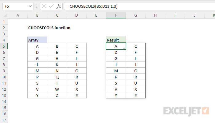
To get columns 1 and 3 from an array, you can use CHOOSECOLS like this:

=CHOOSECOLS(A1:C5,1,3) // columns 1 and 3

To get the same two columns in reverse order:

=CHOOSECOLS(A1:C5,3,1) // columns 3 and 1

CHOOSECOLS will return a #VALUE! error if a requested column number is out of range:

=CHOOSECOLS(A1:C5,4) // returns #VALUE!

With an array constant

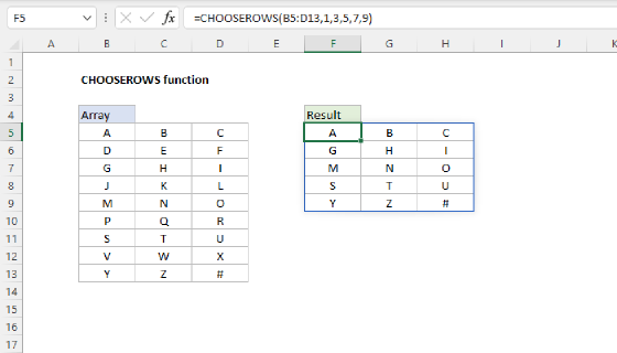
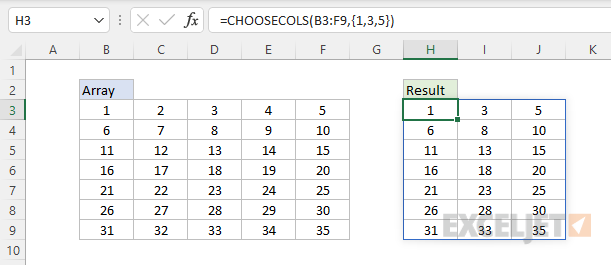
Another option for specifying which columns to return is to use an array constant like {1,2,3} as the second argument (col_num1). In the example below, the formula in H3 is:

=CHOOSECOLS(B3:F9,{1,3,5})

With the array constant {1,3,5} given as the second argument, CHOOSECOLS returns columns 1, 3, and 5:

The array constant provided can be in the form {1,2,3} or {1;2;3}.

With negative column numbers

A nice feature of CHOOSECOLS is that you can use negative column numbers to extract columns from the end of a range. For example, to get the last column of a range, you can use a formula like this:

=CHOOSECOLS(range,-1)

To get the second-to-last column, you can use:

=CHOOSECOLS(range,-2)

To get the last three columns in the order that they appear:

=CHOOSECOLS(range,-3,-2,-1)

You can also mix negative and positive row numbers. To return the first and last columns at the same time:

=CHOOSECOLS(range,1,-1)

With arrays

As seen above, you can use an array constant as the second argument in CHOOSECOLS to specify columns. You can also use an array generated with a formula. For example, in the worksheet below, we use the SEQUENCE function inside CHOOSECOLS to reverse the column order of the range B3:D9 with a formula like this in cell F3:

=CHOOSECOLS(B3:D9,-SEQUENCE(COLUMNS(B3:D9)))

Since the range B3:D9 contains 3 columns, COLUMNS returns 3 and SEQUENCE returns {1;2;3}:

SEQUENCE(3) // returns {1;2;3}

The negative sign before SEQUENCE converts the array to {-1;-2;-3}:

-SEQUENCE(3) // returns {-1;-2;-3}

Simplifying, the final CHOOSECOLS formula looks like this:

=CHOOSECOLS(B3:D9,{-1;-2;-3})

The result is that CHOOSECOLS returns the 3 columns in B3:D9 in reverse order:

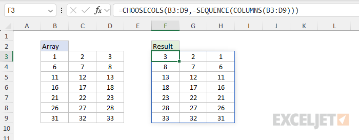
The CHOOSECOLS returns all columns in the array: the last column (-1), the second to last column (-2), and the third to last column (-3).

Notes

• CHOOSECOLS will return a #VALUE error if a column number is out of range.