Summary
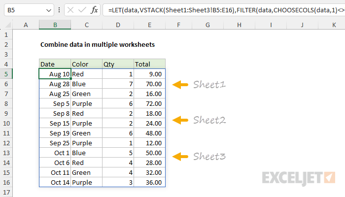
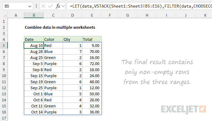
To combine data in multiple worksheets, you can use a formula based on the VSTACK function and the FILTER function. In the example shown, we are combining data on three separate worksheets. The formula in cell B5 is:
=LET(data,VSTACK(Sheet1:Sheet3!B5:E16),FILTER(data,CHOOSECOLS(data,1)<>""))
The result is a single set of data extracted from Sheet1, Sheet2, and Sheet3. The FILTER function is used to remove empty rows.
Generic formula
=LET(data,VSTACK(Sheet1:Sheet3!range),FILTER(data,CHOOSECOLS(data,1)<>""))
Explanation
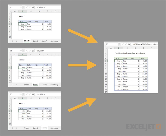
The goal is to combine data from different worksheets with a formula. Note that we are not restructuring the data in any way, we are simply combining data in different worksheets that already have the same structure. At a high level, the formula we are using combines data from multiple sheets with the VSTACK function and removes empty rows with FILTER. The data in the workbook comes from 3 separate worksheets (Sheet1, Sheet2, and Sheet3) and is combined in another worksheet named Summary. The Diagram below provides an overview:
Notice that the range in the formula below is fixed as B5:B16 and some of the rows in this range are empty on each worksheet. This means the solution should also provide a way to remove empty rows in the final result. In the worksheet example above, the formula used to solve this problem in cell B5 looks like this:
=LET(data,VSTACK(Sheet1:Sheet3!B5:E16),FILTER(data,CHOOSECOLS(data,1)<>""))
Let's look at how this formula works step-by-step. The first step is to combine the data, which is done with the VSTACK function.
Note: in this example, we are working with a tiny amount of data in a small number of worksheets so that the problem is easy to understand. However, the same approach will work with larger sets of data in many more worksheets.
Combining data with VSTACK and a 3D reference
The first step in this formula is to combine the data in three separate ranges on three separate sheets. When you have data in "normal" ranges (i.e. data not in a named range or an Excel Table) at a predictable location on multiple worksheets, a nice approach is to use the VSTACK function with a 3D reference like this:
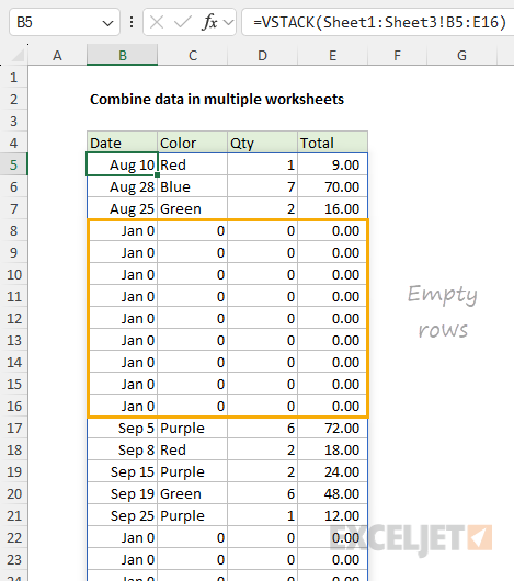
=VSTACK(Sheet1:Sheet3!B5:E16)
The reference "Sheet1:Sheet3!B5:E16" is called a "3D reference". It points to the range B5:E16 on Sheet1 through Sheet3 which, in this case, is Sheet1, Sheet2, and Sheet3. VSTACK retrieves data from the range B5:E16 on each sheet and stacks each range on top of another vertically. This is the core of the formula — the part that does the actual data consolidation.
Note: If you are new to the idea of a 3D reference, this video provides an overview.
This works well, as you can see in the screen below. However, one problem when using a fixed range like this is that the output may contain empty rows, which also appear in the output:
To remove the extra rows, we can use the FILTER function. However, before we do that, it makes sense to store the output from VSTACK in a variable with the LET function. The reason we do this is because we are going to use the same data twice in FILTER. By using a variable, we only need to run the VSTACK operation one time.
LET function
The LET function allows you to name variables inside a formula. This makes more complex formulas easier to read and write. It also improves performance since certain operations only need to run one time. In this case, we use LET to name the output from VSTACK "data" like this:
=LET(data,VSTACK(Sheet1:Sheet3!B5:E16),
VSTACK runs as explained above and the result (the combined ranges) is stored in the variable "data". The next step is to remove the empty rows. For that, we'll use the FILTER function.
Removing empty rows with FILTER
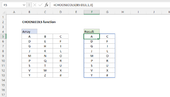
As seen in the screen above, the result from VSTACK (now stored in the variable data) contains empty rows. To remove these empty rows from the final result, we use the FILTER function and the CHOOSECOLS function together like this:
FILTER(data,CHOOSECOLS(data,1)<>"") // remove empty rows
Here, the array in FILTER is provided as data, which was created by LET in the previous step. The logic to remove empty rows is based on the CHOOSECOLS function:
CHOOSECOLS(data,1)<>"" // test column 1
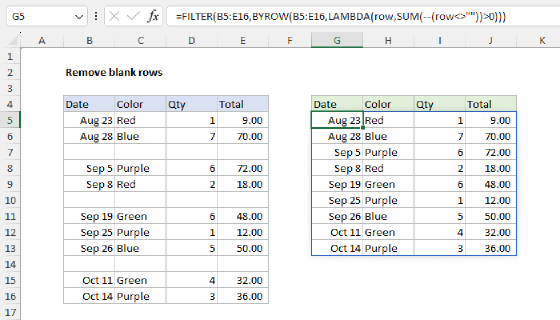
CHOOSECOLS is designed to retrieve one or more specific columns from a larger set of data. In this case, we are asking CHOOSECOLS for the first column in data. Then we use a logical expression to test for "not empty" cells in the column. The result is an array of TRUE and FALSE values, one per row. This array is returned to FILTER as the include argument. When FILTER applies this array of TRUE and FALSE values to data, only the rows associated with TRUE values are returned. The rows associated with FALSE values are discarded. The final result on the summary sheet looks like this:
Note: we are only testing the first column (Date) for empty rows. If you need a more robust test for empty rows, see this example.
Without the LET function
It isn't necessary to use the LET function for this formula, it's just more efficient. Here is the same formula without LET:
=FILTER(VSTACK(Sheet1:Sheet3!B5:E16),CHOOSECOLS(VSTACK(Sheet1:Sheet3!B5:E16),1)<>"")
The overall structure is the same, but notice that we need to run the VSTACK operation twice inside FILTER. With larger amounts of data, this will slow the formula down.
Without a 3D reference
The 3D reference is useful in this problem because the ranges on each sheet are at the same location. As long as this remains true, you can easily expand the 3D reference to include additional sheets. However, there is no requirement that you use a 3D reference. You could refer to each range separately inside VSTACK like this:
=VSTACK(Sheet1!B5:E16,Sheet2!B5:E16,Sheet3!B5:E16)
This works fine, but the approach won't scale well as you add a larger number of sheets.
Using the combined data
Once you have combined the data with the formula above, you can use it normally in other functions. For example, to sum the Total for all rows with a color of "Red", you can use a formula like this:
=SUMIFS(E5:E16,C5:C16,"red")
You can also refer to the spill range B5# to refer to the combined data. For example, to return all rows that have a color of "Red" you can use FILTER like this:
=FILTER(B5#,C5:C16="red")
With Excel Tables
If you are combining data that exists in Excel Tables, this problem is much easier. For example, with the data in this example in three tables (Table1, Table2, and Table3) we can combine the data with a simple VSTACK formula like this:
=VSTACK(Table1,Table2,Table3)
There is usually no need to remove empty rows because Excel Tables automatically expand and contract to fit the data they contain. This means we don't need to use any fancy tricks to figure out how many rows to retrieve, or how many empty rows to remove — we can simply combine data in the tables with VSTACK.
Data in external workbooks
It is possible to combine data in separate external workbooks with VSTACK like this:
VSTACK(Sheet1.xlsx!B5:E16,Sheet2.xlsx!B5:E16,Sheet3.xlsx!B5:E16)
Or, with a 3D reference to a single workbook, like this:
VSTACK([workbook.xlsx]Sheet1:Sheet3!B5:E16)
Note: I have only tested the external links on a single local drive, so results may vary in different environments.