
Summary
Most people never receive proper Excel training and spend years frustrated by the simplest tasks, especially tasks that involve formulas. To use Excel with confidence, you must have a good understanding of formulas and functions. This article introduces the basic concepts you need to know to be proficient with formulas in Excel.
Formulas and functions are the bread and butter of Excel. They drive almost everything interesting and useful you will ever do in a spreadsheet. This article introduces the basic concepts you need to know to be proficient with formulas in Excel. More examples here.
What is a formula?
A formula in Excel is an expression that returns a specific result. For example:
=1+2 // returns 3

=6/3 // returns 2
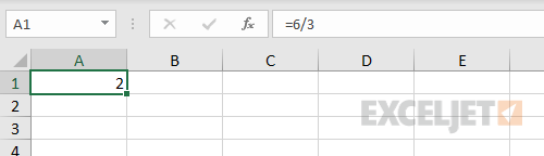
Note: all formulas in Excel must begin with an equals sign (=).
Cell references
In the examples above, values are "hardcoded". That means results won't change unless you edit the formula again and change a value manually. Generally, this is considered bad form, because it hides information and makes it harder to maintain a spreadsheet.
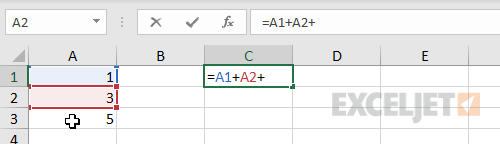
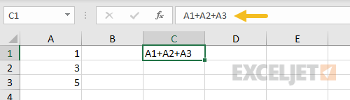
Instead, use cell references so values can be changed at any time. In the screen below, C1 contains the following formula:
=A1+A2+A3 // returns 9
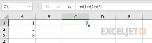
Notice because we are using cell references for A1, A2, and A3, these values can be changed at any time and C1 will still show an accurate result.
All formulas return a result
All formulas in Excel return a result, even when the result is an error. Below a formula is used to calculate percent change. The formula returns a correct result in D2 and D3, but returns a #DIV/0! error in D4, because B4 is empty:
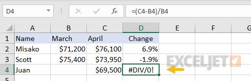
There are different ways of handling errors. In this case, you could provide the missing value in B4, or "catch" the error with the IFERROR function and display a more friendly message (or nothing at all).
Copy and paste formulas
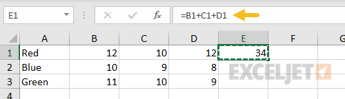
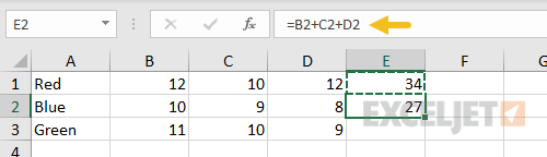
The beauty of cell references is that they automatically update when a formula is copied to a new location. This means you don't need to enter the same basic formula again and again. In the screen below, the formula in E1 has been copied to the clipboard with Control + C:
Below: formula pasted to cell E2 with Control + V. Notice cell references have changed:
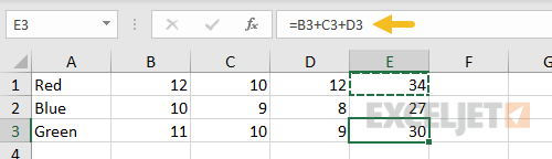
Below is the formula pasted to E3. Cell addresses are updated again:
Relative and absolute references
The cell references above are called relative references. This means the reference is relative to the cell it lives in. The formula in E1 above is:
=B1+C1+D1 // formula in E1
Literally, this means "cell 3 columns left "+ "cell 2 columns left" + "cell 1 column left". That's why, when the formula is copied down to cell E2, it continues to work in the same way.
Relative references are extremely useful, but there are times when you don't want a cell reference to change. A cell reference that won't change when copied is called an absolute reference. To make a reference absolute, use the dollar symbol ($):
=A1 // relative reference
=$A$1 // absolute reference
For example, in the screen below, we want to multiply each value in column D by 10, which is entered in A1. By using an absolute reference for A1, we "lock" that reference so it won't change when the formula is copied to E2 and E3:
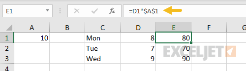
Here are the final formulas in E1, E2, and E3:
=D1*$A$1 // formula in E1
=D2*$A$1 // formula in E2
=D3*$A$1 // formula in E3
Notice the reference to D1 updates when the formula is copied, but the reference to A1 never changes. Now we can easily change the value in A1, and all three formulas recalculate. Below the value in A1 has changed from 10 to 12:
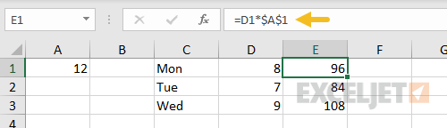
This simple example also shows why it doesn't make sense to hardcode values into a formula. By storing the value in A1 in one place, and referring to A1 with an absolute reference, the value can be changed at any time and all associated formulas will update instantly.
Tip: you can toggle between relative and absolute syntax with the F4 key.
How to enter a formula
To enter a formula:
- Select a cell
- Enter an equals sign (=)
- Type the formula, and press enter.
Instead of typing cell references, you can point and click, as seen below. Note references are color-coded:
All formulas in Excel must begin with an equals sign (=). No equals sign, no formula:
How to change a formula
To edit a formula, you have 3 options:
- Select the cell, edit in the formula bar
- Double-click the cell, edit directly
- Select the cell, press F2, and edit directly
No matter which option you use, press Enter to confirm changes when done. If you want to cancel, and leave the formula unchanged, click the Escape key.
Video: 20 tips for entering formulas
What is a function?
Working in Excel, you will hear the words "formula" and "function" used frequently, sometimes interchangeably. They are closely related, but not exactly the same. Technically, a formula is any expression that begins with an equals sign (=).
A function, on the other hand, is a formula with a special name and purpose. In most cases, functions have names that reflect their intended use. For example, you probably know the SUM function already, which returns the sum of given references:
=SUM(1,2,3) // returns 6
=SUM(A1:A3) // returns A1+A2+A3
The AVERAGE function, as you would expect, returns the average of given references:
=AVERAGE(1,2,3) // returns 2
The MIN and MAX functions return minimum and maximum values, respectively:
=MIN(1,2,3) // returns 1
=MAX(1,2,3) // returns 3
Excel contains hundreds of specific functions. To get started, see 101 Key Excel functions.
Function arguments
Most functions require inputs to return a result. These inputs are called "arguments". A function's arguments appear after the function name, inside parentheses, separated by commas. All have a name, and an opening and closing parentheses (). The inputs inside the parentheses are called "arguments".The pattern looks like this:
=NAME(argument1,argument2,argument3)
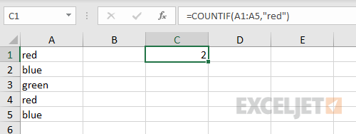
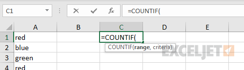
For example, the COUNTIF function counts cells that meet criteria, and takes two arguments, range and criteria:
=COUNTIF(range,criteria) // two arguments
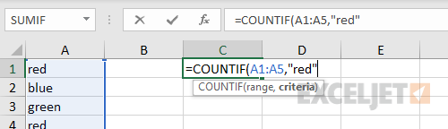
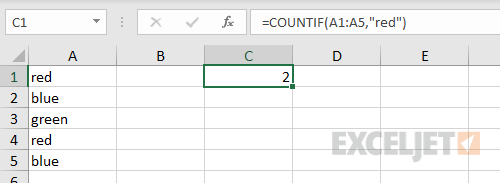
In the screen below, range is A1:A5 and criteria is "red". The formula in C1 is:
=COUNTIF(A1:A5,"red") // returns 2
Video: How to use the COUNTIF function
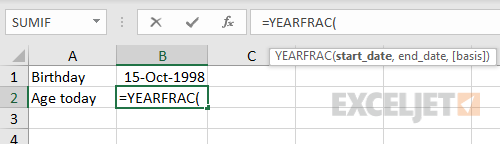
Not all arguments are required. Arguments shown in square brackets [ ] are optional. For example, the YEARFRAC function returns the fractional number of years between a start date and an end date and takes 3 arguments:
=YEARFRAC(start_date,end_date,[basis])
Start_date and end_date are required arguments, basis is an optional argument. See below for an example of how to use YEARFRAC to calculate current age based on birthdate.
How to enter a function
If you know the name of the function, just start typing. Here are the steps:
- Enter an equals sign (=) and start typing. Excel will make a list of matching functions based as you type:
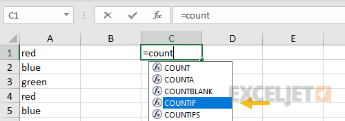
When you see the function you want in the list, use the arrow keys to select (or just keep typing).
- Type the Tab key to accept a function. Excel will complete the function:
- Fill in required arguments:
- Press Enter to confirm formula:
Combining functions (nesting)
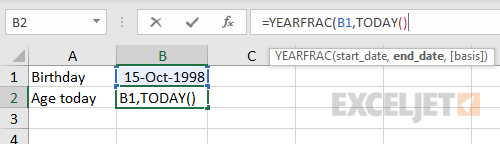
Many Excel formulas use more than one function, and functions can be "nested" inside each other. For example, below we have a birthdate in B1 and we want to calculate the current age in B2:

The YEARFRAC function will calculate years with a start date and end date:
We can use B1 for the start date, and then use the TODAY function to supply the end date:
When we press Enter to confirm, we get current age based on today's date:
=YEARFRAC(B1,TODAY())
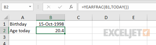
Notice we are using the TODAY function to feed an end date to the YEARFRAC function. In other words, the TODAY function can be nested inside the YEARFRAC function to provide the end date argument. We can take the formula one step further and use the INT function to chop off the decimal value:
=INT(YEARFRAC(B1,TODAY()))
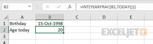
Here, the original YEARFRAC formula returns 20.4 to the INT function, and the INT function returns a final result of 20.
Notes:
- The screens above were created on February 22, 2019.
- Nested IF functions are a classic example of nesting functions.
- The TODAY function is a rare Excel function with no required arguments.
Key takeaway: The output of any formula or function can be fed directly into another formula or function.
Math Operators
The table below shows the standard math operators available in Excel:
| Symbol | Operation | Example |
|---|---|---|
| + | Addition | =2+3=5 |
| - | Subtraction | =9-2=7 |
| * | Multiplication | =6*7=42 |
| / | Division | =9/3=3 |
| ^ | Exponentiation | =4^2=16 |
| () | Parentheses | =(2+4)/3=2 |
Logical operators
Logical operators provide support for comparisons such as "greater than", "less than", etc. The logical operators available in Excel are shown in the table below:
| Operator | Meaning | Example |
|---|---|---|
| = | Equal to | =A1=10 |
| <> | Not equal to | =A1<>10 |
| > | Greater than | =A1>100 |
| < | Less than | =A1<100 |
| >= | Greater than or equal to | =A1>=75 |
| <= | Less than or equal to | =A1<=0 |
Video: How to build logical formulas
Order of operations
When solving a formula, Excel follows a sequence called "order of operations". First, any expressions in parentheses are evaluated. Next Excel will solve for any exponents. After exponents, Excel will perform multiplication and division, then addition and subtraction. If the formula involves concatenation, this will happen after standard math operations. Finally, Excel will evaluate logical operators, if present.
- Parentheses
- Exponents
- Multiplication and Division
- Addition and Subtraction
- Concatenation
- Logical operators
Tip: you can use the Evaluate feature to watch Excel solve formulas step-by-step.
Convert formulas to values
Sometimes you want to get rid of formulas and leave only values in their place. The easiest way to do this in Excel is to copy the formula, then paste, using Paste Special > Values. This overwrites the formulas with the values they return. You can use a keyboard shortcut for pasting values, or use the Paste menu on the Home tab on the ribbon.
Video: Paste Special Shortcuts
What's next?
Below are guides to help you learn more about Excel's formulas and functions. We also offer online video training.
- 29 tips for working with formulas and functions (video version here)
- 500 formula examples with full explanations
- 101 important Excel functions
- Guide to all Excel functions (work in progress)
- Excel formula errors (examples and fixes)
- Formula criteria - 50 examples
- Formulas for conditional formatting
- How to use F9 to debug a formula (video)
- Excel formula errors and fixes (video)


