=SUMIFS(sum_range, range1, criteria1, [range2], [criteria2], ...)- sum_range - The range to be summed.
- range1 - The first range to evaluate.
- criteria1 - The criteria to use on range1.
- range2 - [optional] The second range to evaluate.
- criteria2 - [optional] The criteria to use on range2.
Using the SUMIFS function
The SUMIFS function sums numbers in Excel when they meet one or more specific conditions. SUMIFS is one of Excel's most widely used functions, and you will see it in all kinds of spreadsheets that calculate conditional sums based on dates, text, or numbers. Although a common function, SUMIFS has a unique syntax that splits logical conditions into two parts, making it different from many other Excel functions. As a result, the task of defining criteria in SUMIFS can be a bit tricky. Also note that SUMIFS uses "AND logic". To be included in the final result, all conditions must be TRUE.
Key features
- Sums values that meet one or more conditions
- Each new condition requires a separate range and criteria.
- Works with dates, text, and numbers
- Supports comparison operators (>, <, <>, =) and wildcards (*, ?)
- To be included in the final result, all conditions must be TRUE.
- All ranges must be the same size, or SUMIFS will return a #VALUE! error.
- Available in all Excel versions since Excel 2007
Unlike most other Excel functions, SUMIFS requires an actual range for sum/criteria ranges. If you try to use an array, Excel will not let you enter the formula. For details, see the example below.
Table of Contents
- Syntax
- Basic Example
- Applying Criteria
- Criteria in another cell
- Not equal to
- Blank cells
- Dates
- Wildcards
- OR logic
- Summary Table
- Array Problem
- Limitations
- Notes
Syntax
The syntax for the SUMIFS function depends on the criteria being evaluated. Each condition is provided with a separate range and criteria. The generic syntax for SUMIFS looks like this:
=SUMIFS(sum_range,range1,criteria1) // 1 condition
=SUMIFS(sum_range,range1,criteria1,range2,criteria2) // 2 conditions
Note that the sum_range always comes first. This is the range of cells to sum. Each condition is provided as a pair of range/criteria arguments. The first formula above defines one condition and the second defines two. Additional conditions are defined by additional range/criteria pairs.
Basic Example
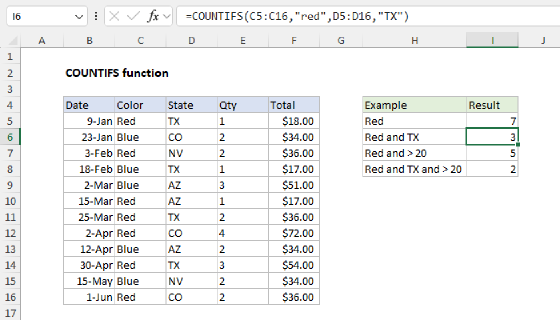
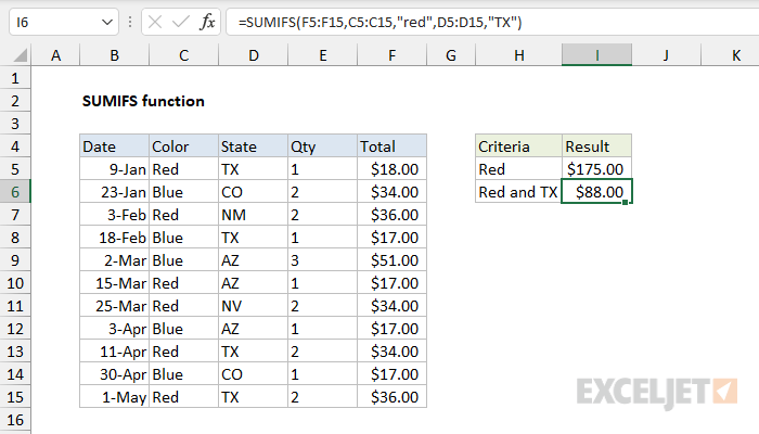
The worksheet below contains simple order data. We use SUMIFS to perform three calculations:
- Sum values where the color is Red.
- Sum values where the color is Red and the state is TX.
- Sum values where the color is Red, the state is TX, and the total is >20.
The three formulas in I5:I7 look like this:
=SUMIFS(F5:F16,C5:C16,"red") // Red
=SUMIFS(F5:F16,C5:C16,"red",D5:D16,"TX") // Red and TX
=SUMIFS(F5:F16,C5:C16,"red",D5:D16,"TX",F5:F16,">20") // Red and TX and >20
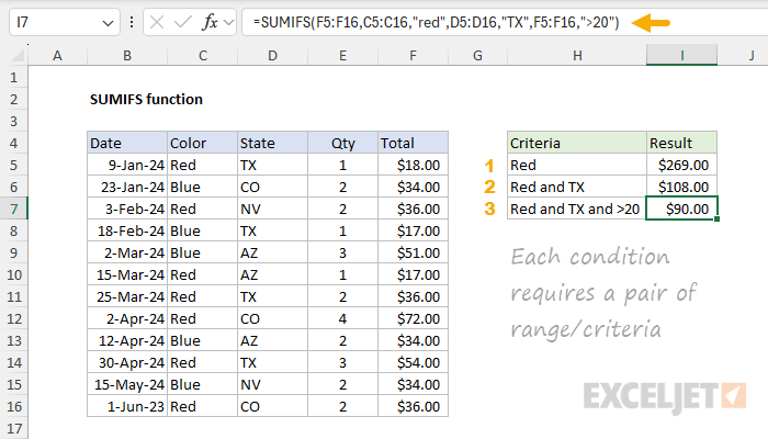
There are a few things worth noting in the formulas above:
- An equal sign (=) is not needed with "is equal to" criteria (i.e. use "red" not "=red").
- SUMIFS is not case-sensitive, so "red" and "Red" will return the same results.
- Numbers must appear in quotes ("") when used with operators (i.e. ">20").
- SUMIFS always uses "AND logic". All conditions must be true.
Note that the syntax for the criteria argument in SUMIFS is somewhat unusual in Excel. Instead of simply entering >20 as the criteria, you must enter ">20" in double quotes. If you don't quote values as required, Excel will not let you enter the formula. See below for more examples of this syntax.
Applying Criteria
The SUMIFS function supports logical operators (>,<,<>,=) and wildcards (*,?) for partial matching. The tricky part is the syntax needed to apply the criteria. This is because SUMIFS is in a group of eight functions that split logical criteria into two parts: range and criteria. Because of this design, operators must be enclosed in double quotes (""). The table below shows the syntax required for a variety of criteria:
| Target | Criteria |
|---|---|
| Cells greater than 75 | ">75" |
| Cells equal to 100 | 100 or "100" |
| Cells less than or equal to 100 | "<=100" |
| Cells equal to "Red" | "red" |
| Cells not equal to "Red" | "<>red" |
| Cells that are blank "" | "" |
| Cells that are not blank | "<>" |
| Cells that begin with "X" | "x*" |
| Cells equal to A1 | A1 |
| Cells less than A1 | "<"&A1 |
| Cells less than today | "<"&TODAY() |
Notice the last two examples involve concatenation with the ampersand (&) character. Any time you use a value from another cell or the result of a formula with a logical operator like "<", you must concatenate. This is because Excel needs to evaluate cell references and formulas first before the value can used with an operator.
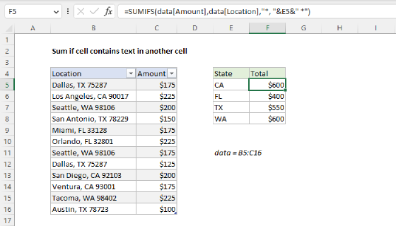
Criteria in another cell
It is often convenient to put criteria in another cell and then refer to this cell inside your formula. This makes it easy to change criteria later without editing the original formula. For example, you can sum cells in a range equal to the value in A1 like this:
=SUMIFS(sum_range,range,A1)
When a condition requires an operator, you must concatenate the cell reference to the operator. For example, to sum cells in a range greater than A1, use a formula like this:
=SUMIFS(sum_range,range,">"&A1)
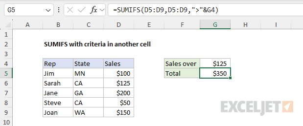
Note we are joining the ">" operator to cell A1 with an ampersand (&) character. In the worksheet below, SUMIFS has been configured to return the sum of all sales over the value in G4. Notice the greater than operator (>), which is text, must be enclosed in quotes. The formula in G5 is:
=SUMIFS(D5:D9,D5:D9,">"&G4) // sum if greater than G4
Don't enclose cell references in double quotes like "A1". Doing so will convert them to text.
Not equal to
To express "not equal to" criteria, use the "<>" operator surrounded by double quotes (""). For example, use "<>red" for "not red", and "<>blue" for "not blue", as seen in the worksheet below:
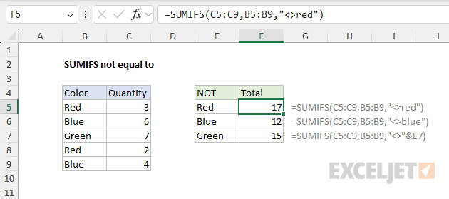
=SUMIFS(C5:C9,B5:B9,"<>red") // not red
=SUMIFS(C5:C9,B5:B9,"<>blue") // not blue
=SUMIFS(C5:C9,B5:B9,"<>"&E7) // not E7
Note the following:
- In the last formula, we use E7 directly, so we need to concatenate like "<>"&E7.
- Do not use quotes around the cell reference.
- SUMIFS is not case-sensitive, so "red", "RED", and "Red" will return the same result.
Blank cells
SUMIFS can calculate sums based on whether cells are blank or not blank. Use an empty string ("") to target blank cells and the "not equal to" operator ("<>") to target cells that are not blank. In the worksheet below, SUMIFS is used to sum the amounts in column C depending on whether column D contains "x" or is empty:
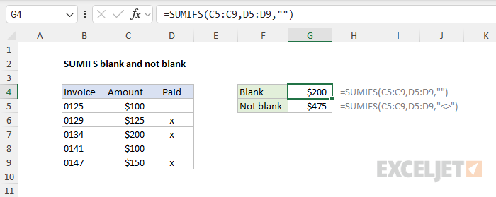
=SUMIFS(C5:C9,D5:D9,"") // blank
=SUMIFS(C5:C9,D5:D9,"<>") // not blank
In the second formula, any value in a cell will cause SUMIFS to sum the amount. To be more precise, you can use a formula like this that sums values only when column D contains an "x":
=SUMIFS(C5:C9,D5:D9,"x")
Dates
In Excel, dates are serial numbers, so you can use operators like <,>, <=, >= with dates like any other number. The tricky part about using dates in SUMIFS conditions is entering the dates in a way that Excel will understand. The most reliable way to do this is to refer to a valid date in another cell or use the DATE function. The example below shows both methods:
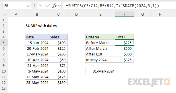
The formulas in F5:F8 are as follows:
=SUMIFS(C5:C12,B5:B12,"<"&DATE(2024,3,1))
=SUMIFS(C5:C12,B5:B12,">="&DATE(2024,3,31))
=SUMIFS(C5:C12,B5:B12,">"&E10)
=SUMIFS(C5:C12,B5:B12,">="&DATE(2024,5,1),B5:B12,"<="&DATE(2024,5,31))
Note the following:
- When using a cell reference, you must concatenate the reference to an operator like ">"&E10.
- In general, it's best to avoid hardcoding a date into a formula and refer to a date in another cell instead.
- Referring to a date in another cell makes it easy to change the date without editing the formula.
Pro tip: Avoid hard-coding a date into a formula. Instead, put the date in a cell, then reference that cell in your formula. This makes the worksheet more useful since you can easily see the date being used and change the date when needed without editing the formula.
Wildcards
The SUMIFS function supports three wildcards you can use in criteria:
- Asterisk (*) - match zero or more characters
- Question mark (?) - match any one character
- Tilde (~) - an escape character to match a literal wildcard
The worksheet below shows how wildcards can be used with the SUMIFS function. The formulas in F5:F8 apply the criteria described in column E.
=SUMIFS(C5:C11,B5:B11,"mi*") // begins with "mi"
=SUMIFS(C5:C11,B5:B11,"*ota") // ends with "ota"
=SUMIFS(C5:C11,B5:B11,"????") // contains 4 characters
=SUMIFS(C5:C11,B5:B11,"*~?") // ends with "?"
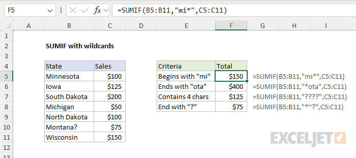
Note the last formula in F8 uses "~?" to match a question mark (?) that occurs at the end of "Montana?" in cell C10. The tilde (~) is an escape character that allows you to find a literal wildcard. To match a question mark (?), use "~?"; to match an asterisk(), use "~*"; and to match a tilde (~), use "~~". The table below shows more examples of how wildcards can be used:
| Pattern | Behavior | Will match |
|---|---|---|
| ? | Any one character | "A", "B", "c", "z", etc. |
| ?? | Any two characters | "AA", "AZ", "zz", etc. |
| ??? | Any three characters | "Jet", "AAA", "ccc", etc. |
| * | Any characters | "apple", "APPLE", "A100", etc. |
| *th | Ends in "th" | "bath", "fourth", etc. |
| c* | Starts with "c" | "Cat", "CAB", "cindy", "candy", etc. |
| ?* | At least one character | "a", "b", "ab", "ABCD", etc. |
| ???-?? | Five characters with a hyphen | "ABC-99","100-ZT", etc. |
| *~? | Ends with a question mark | "Hello?", "Anybody home?", etc. |
| xyz | Contains "xyz" | "code is XYZ", "100-XYZ", "XyZ90", etc. |
Note: wildcards only work with text, not numbers.
OR logic
The SUMIFS function is designed to apply multiple conditions with "AND logic," so there is no obvious way to sum cells with "OR logic". However, one workaround is to provide the criteria as an array constant like {"red","blue}, and then nest the SUMIFS formula inside the SUM function like this:
=SUM(SUMIFS(sum_range,range,{"red","blue"})) // red or blue
The formula above will sum cells in sum_range when cells in range contain "red" or "blue". Essentially, SUMIFS returns two sums, one for "red" and one for "blue", and the SUM function returns the sum of the sums. For more details, see this example.
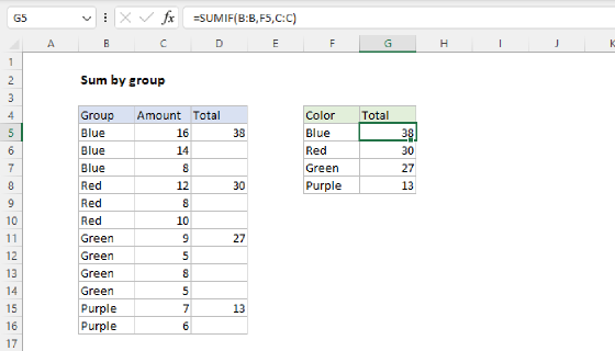
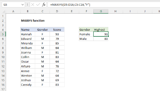
Summary Table
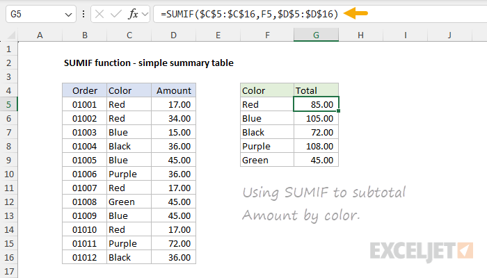
You can use SUMIFS to create a simple summary table. In the worksheet below, we have a list of unique colors in F5:F9. The goal is to subtotal the amounts in column D by color. The formula in cell G5, copied down, is:
=SUMIFS($D$5:$D$16,$C$5:$C$16,F5)
Notice that the range and the sum_range are locked as absolute references to prevent changes as the formula is copied down the column. If you are using Excel 2021 or later, you can generate all totals at once with a dynamic array formula like this:
=SUMIFS(D5:D16,C5:C16,F5:F9)
We don't need the absolute references in this case because a single formula creates all results. You can go one step further by using the UNIQUE function in cell F5 to get a list of unique colors, then referring to the spill range directly like this:
=SUMIFS(D5:D16,C5:C16,F5#)
In Excel 365, you can also use the new GROUPBY function to create a summary table.
Array Problem
Note: For more advanced use cases, this is an important limitation in what SUMIFS can do.
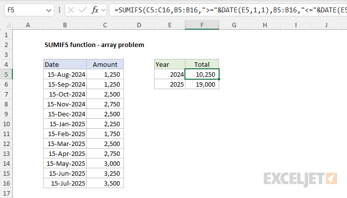
One of the more tricky limitations of SUMIFS is that it won't allow an array for a range argument. To understand the problem, consider the worksheet below, where we have 12 dates in column B and 12 amounts in column C. The goal is to create a formula to sum the amounts by year. We can do that with the following SUMIFS formula:
=SUMIFS(C5:C16,B5:B16,">="&DATE(E5,1,1),B5:B16,"<="&DATE(E5,12,31))
Note: I would normally use absolute references for the two ranges so that the formula can be copied down without changes, but I have left the addresses relative here so they are easier to read.
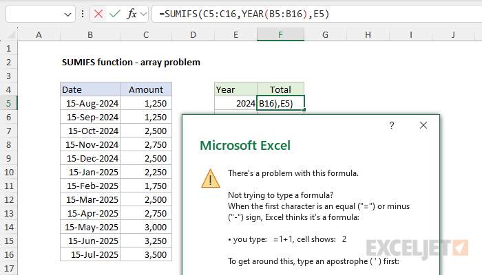
This formula works fine, but it's a little complicated. If you have some experience with Excel formulas, you might think you can use SUMIFS and YEAR together in a clever formula like this:
=SUMIFS(C5:C16,YEAR(B5:B16),E5)
The idea is to extract the year from the dates in column B with the YEAR function, and then use 2024 (in cell E5) for the criteria. This would be cool if it worked. However, Excel won't even let you enter this formula. If you try, you'll get a generic "There's a problem with your formula" error:
The problem is that SUMIFS requires a proper range for the range argument, but YEAR(B5:B16) will return an array like this:
{2024;2024;2024;2024;2024;2025;2025;2025;2025;2025;2025;2025}
To be clear, using YEAR like this works fine in most other formulas. However, SUMIFS is not programmed to handle arrays, so it won't work. How can we work around this problem? One nice alternative is to switch to the SUMPRODUCT function and use a formula like this:
=SUMPRODUCT(sum_range,--(range=criteria))
If we modify the pattern above to fit the workbook example, we get the following:
=SUMPRODUCT(C5:C16,--(YEAR(B5:B16)=E5))
This formula is quite a bit simpler than the SUMIFS formula above. It's a good example of how SUMPRODUCT can often solve a tricky problem in a clever and elegant formula.
Remember: If you try to provide an array for a range, you won't be able to enter the formula because Excel will display a "There's a problem with your formula" error dialog. The "array problem" is not mentioned explicitly.
Limitations
The SUMIFS function has several limitations you should be aware of:
- Conditions in SUMIFS are joined by AND logic. In other words, all conditions must be TRUE in order for a cell to be included in a sum. To sum cells with OR logic, you can use a workaround in simple cases.
- All ranges must be the same size. If you supply ranges that don't match, you'll get a #VALUE error. See example here.
- The SUMIFS function requires actual ranges for all range arguments; you can't use an array. This means you can't do things like extract the year from dates inside the SUMIFS function. To alter values that appear in a range argument before applying criteria, the SUMPRODUCT function is a flexible solution.
- SUMIFS is not case-sensitive. To sum values based on a case-sensitive condition, you can use a formula based on the SUMPRODUCT function with the EXACT function.
- If you reference a range in an external workbook, SUMIFS requires that the workbook be open to calculate a result. If the external workbook is not open, you will see a #VALUE! error. As a workaround, you can switch to the SUMPRODUCT function, which does not have this limitation. The syntax will look like this: =SUMPRODUCT(--(criteria_range1=criteria1), --(criteria_range2=criteria2) ... , sum_range). See this page for details.
- SUMIFS has some other quirks, which are detailed in this article.
The most common way to work around most of these limitations is to use the SUMPRODUCT function.
Notes
- Multiple conditions are applied using AND logic, i.e., condition 1 AND condition 2, etc.
- All ranges must be the same size. If you supply ranges that don't match, you'll get a #VALUE error.
- Non-numeric criteria must be enclosed in double quotes (i.e., "<100", ">32", "TX").
- Cell references in criteria are not enclosed in quotes, i.e., "<"&A1
- The wildcard characters "?" and "" can be used in criteria. A question mark (?) matches any one character, and an asterisk () matches any sequence of characters (zero or more).
- To match a literal question mark(?) or asterisk (), use a tilde (~) like (~?, ~).
- SUMIFS requires a range; you can't substitute an array.