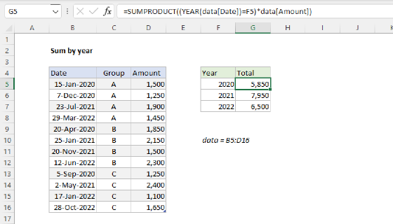
Summary
To sum values by week number, you can use a formula based on the SUMIFS function and the WEEKNUM function. In the example shown, the formula in G5 is:
=SUMIFS(data[Amount],data[Week],G5)
where data is an Excel Table in the range B5:E16, and the week numbers in column E are generated with the WEEKNUM function.
Generic formula
=SUMIFS(sum_range,week_range,week)
Explanation
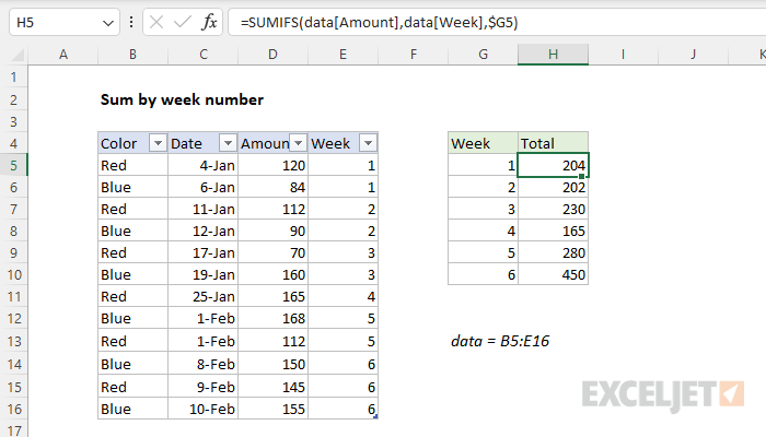
In this example, the goal is to sum the amounts in column D by week number, using the dates in column C to determine the week number. The week numbers in column G are manually entered. The final results should appear in column H. All data is in an Excel Table named data in the range B5:E16. This problem can be solved with the SUMIFS function and the WEEKNUM function as explained below.
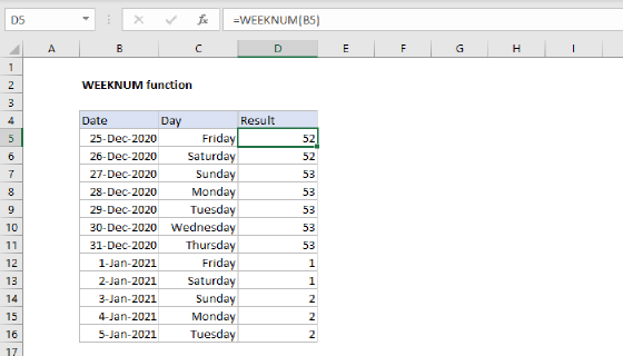
WEEKNUM function
The first step in this problem is to generate a week number for each date in column B. In the table shown, column E is a helper column with week numbers generated with the WEEKNUM function. The formula in E5, copied down, is:
=WEEKNUM([@Date],2) // get week number
Note: because we are using an Excel Table to hold the data, we automatically get the structured reference seen above. The reference [@Date] means: current row in Date column. If you are new to structured references, see this short video: Introduction to structured references.
The WEEKNUM function takes a valid Excel date as the first argument. The second argument is called return_type and indicates the day of the week that week numbers should begin. Setting return_type to 2 specifies that week numbers should begin on Mondays.
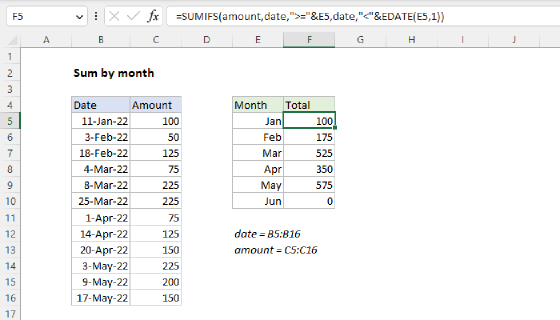
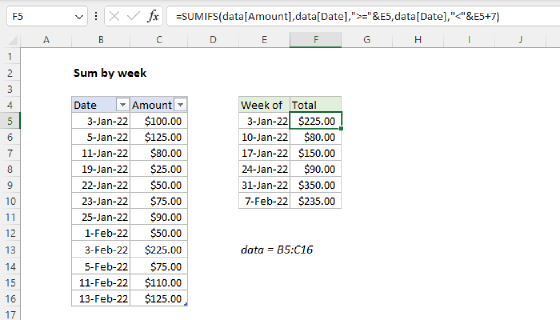
SUMIFS solution
The next step in the problem is to add up the amounts in column D using the week numbers in column E. This can easily be done with the SUMIFS function. The SUMIFS function is designed to sum values in ranges conditionally based on multiple criteria. The signature of the SUMIFS function looks like this:
=SUMIFS(sum_range,range1,criteria1,range2,criteria2,...)
Notice the sum_range comes first, followed by range/criteria pairs. Each range/criteria pair of arguments represents another condition.
In this case, we need to configure SUMIFS to sum values by week number using just one condition: we need to check the week number in column E for a match in the week number in column G. We start off with the sum_range:
=SUMIFS(data[Amount]
Next, we add criteria as a range/criteria pair, where criteria_range1 is the date column, and criteria1 is the week number in column G:
=SUMIFS(data[Amount],data[Week],G5)
Note: we don't use data[Week]=G5 because SUMIFS is in a group of eight functions that split formula criteria into two parts.
As the formula is copied down, we get a total for each week number in column G.
Dynamic array solution
In the latest version of Excel, which supports dynamic array formulas, it is possible to create a single all-in-one formula that builds the entire summary table, including headers, like this:
=LET(
weeks,WEEKNUM(+data[Date],2),
amounts,data[Amount],
uweeks,UNIQUE(weeks),
totals, BYROW(uweeks, LAMBDA(r, SUM((weeks=r)*amounts))),
VSTACK({"Week","Total"},HSTACK(uweeks, totals))
)
The LET function is used to assign four intermediate variables: weeks, uweeks, totals, and totals. The value for weeks is created like this:
WEEKNUM(+data[Date],2) // get all weeks
Here, the WEEKNUM function is used to fetch week numbers for all dates in data[Date]. Because the table contains 12 rows, the result is an array with 12 week numbers like this:
{1;1;2;2;3;3;4;5;5;6;6;6}
Note: the + operator before data[Date] is a workaround for some Excel functions that don't spill properly.
In the next line, we assign a value to amounts like this:
amounts,data[Amount]
Note: Technically, we could just use the reference to data[Amount], but defining a variable here keeps all worksheet references at the top of the formula where they can be easily changed.
In our summary table, we want a list of unique week numbers, so we define uweeks (unique weeks) with the UNIQUE function like this:
UNIQUE(weeks) // get unique week numbers
From the 12 week numbers seen above, the UNIQUE function returns just 6 unique numbers:
{1;2;3;4;5;6} // unique week numbers
Note: You could run these week numbers through the SORT function to ensure that weeks are in the correct order, but a better approach would be to SORT the dates themselves before extracting the week numbers. This is because week numbers in Excel can vary in the early part of a year. For example, the first few days of a year could be in week number 53.
At this point, we are ready to sum amounts by week number. We do this with the BYROW function, which calculates the sums and assigns the result to the variable totals for each week, like this:
totals, BYROW(uweeks, LAMBDA(r, SUM((weeks=r)*amounts)))
BYROW runs through the uweeks values row by row. At each row, it applies this calculation:
LAMBDA(r, SUM((weeks=r)*amounts))
The value for r is the week number in the "current" row. Inside the SUM function, this value is compared to weeks. Since weeks contains all 12 values, the result is an array with 12 TRUE and FALSE results. The TRUE and FALSE values are multiplied by amounts. The math operation automatically converts the TRUE and FALSE values to 1s and 0s, and the zeros effectively "cancel" the values in week numbers not equal to r. The SUM function then sums the resulting array and returns the result. When BYROW is finished, we have an array with six sums like this:
{204;202;230;165;280;450} // totals
This is the value assigned to totals.
Finally, the HSTACK and VSTACK functions are used to assemble a complete table:
VSTACK({"Week","Total"},HSTACK(uweeks, totals))
At the top of the table, the array constant {"Week","Total"} creates a header row. The HSTACK function combines uweeks and totals horizontally, and VSTACK combines the header row and the data to make the final table. The final result spills into multiple cells on the worksheet.