UNIQUE Function

The UNIQUE function extracts a list of unique values from a range or array. The result is a dynamic array that spills onto the worksheet, automatically updating when source data changes.

UNIQUE is often combined with other dynamic array functions like FILTER and SORT. For example, you can filter data before extracting unique values, or sort the results alphabetically. Use the ROWS function or COUNTA function to count the unique values returned by UNIQUE.

Note that UNIQUE won't automatically adjust the source range if data is added or deleted. To use UNIQUE with a range that automatically resizes to fit the data, use an Excel Table or a dynamic range created with TRIMRANGE or the dot operator.

Video: The UNIQUE function

Key features

• Extracts unique values from a range or array automatically.
• Returns a dynamic array that updates when source data changes.
• Case-insensitive: "APPLE", "Apple", and "apple" are treated as the same value.
• Set exactly_once to TRUE to return only values that appear once (distinct values).
• Set by_col to TRUE to extract unique values from horizontal data.
• Only works with adjacent columns; use CHOOSECOLS or FILTER for non-adjacent columns.

Table of contents

• Basic usage
• Unique values
• Unique values by column
• Sort unique values
• Unique rows
• Distinct values
• Unique values ignore blanks
• Unique values with criteria
• Count unique values
• Unique values by count
• Unique with non-adjacent columns
• Notes

Basic usage

Using the UNIQUE function is straightforward. Just provide a range or array:

=UNIQUE(A1:A10) // unique values from A1:A10

Here are a few variations, which are explained in more detail below:

=UNIQUE(A1:B10) // unique rows from two columns
=UNIQUE(A1:E1,TRUE) // unique values from horizontal range
=UNIQUE(A1:A10,,TRUE) // unique values that appear exactly once
=SORT(UNIQUE(A1:A10)) // unique values, sorted

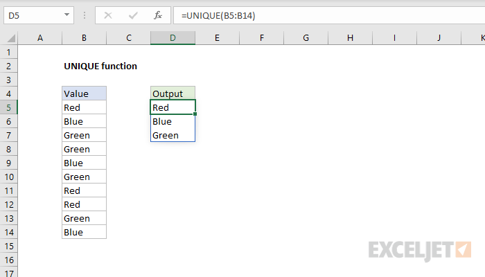
Unique values

In the worksheet below, the goal is to extract a list of unique colors from the range B5:B16. The formula in D5 is:

=UNIQUE(B5:B16)

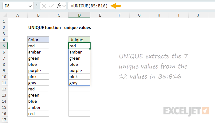
The UNIQUE function evaluates the 12 values in B5:B16 and returns the 7 unique colors. The result spills into the range D5:D11 automatically. If any data in B5:B16 changes, the output from UNIQUE updates immediately.

For more details, see Unique values.

Unique values by column

By default, UNIQUE compares values by row. To extract unique values from horizontal data (arranged in columns), set by_col to TRUE. In the worksheet below, the goal is to extract unique colors from the range C4:I4. The formula in C6 is:

=UNIQUE(C4:I4,TRUE)

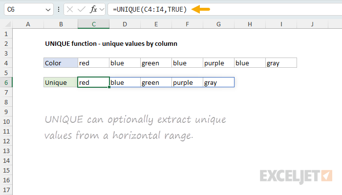
With by_col set to TRUE, UNIQUE compares values across columns instead of down rows. The result spills horizontally, returning the 5 unique colors: red, blue, green, purple, and gray. To convert the horizontal result to a vertical list, wrap the formula with TRANSPOSE:

=TRANSPOSE(UNIQUE(C4:I4,TRUE))

Sort unique values

A common pattern is to combine UNIQUE with SORT to return unique values in alphabetical or numerical order. In the worksheet below, the goal is to extract unique colors and sort them alphabetically. The formula in D5 is:

=SORT(UNIQUE(B5:B16))

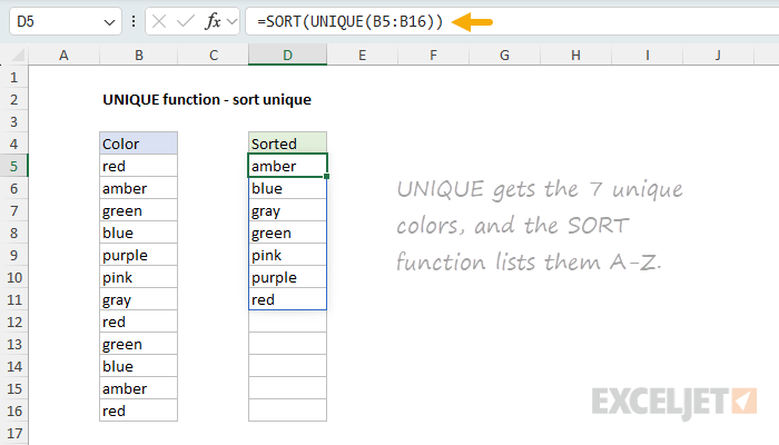
Working from the inside out, UNIQUE extracts the 7 unique colors, then SORT arranges them in ascending order (A to Z). To sort in descending order (Z to A), add -1 as the third argument to SORT:

=SORT(UNIQUE(B5:B16),,-1)

Unique rows

UNIQUE can extract unique rows from multi-column data. In the worksheet below, the goal is to extract unique rows from the range B5:C15, which contains Group and Color columns. The formula in E5 is:

=SORT(UNIQUE(B5:C15))

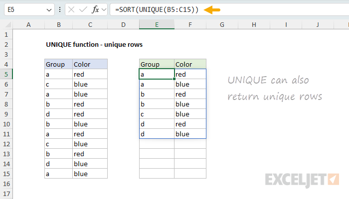
By default, UNIQUE compares values by row, so no special configuration is needed. The UNIQUE function evaluates all 11 rows and returns the 7 unique combinations of Group and Color. The SORT function then sorts the result by the first column (Group). SORT is optional and can be removed if sorting isn't needed.

For more details, see Unique rows.

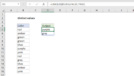
Distinct values

The exactly_once argument controls how UNIQUE handles repeating values. By default, UNIQUE returns all unique values regardless of how many times they appear. Set exactly_once to TRUE to return only values that appear exactly once in the data. In the worksheet below, the goal is to extract colors that appear only once. The formula in D5 is:

=UNIQUE(B5:B16,FALSE,TRUE)

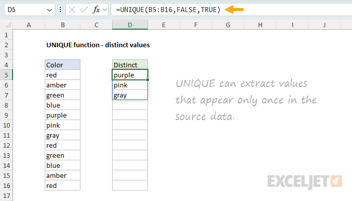
Because exactly_once is TRUE, UNIQUE returns only the 3 values that appear once: "purple", "pink", and "gray". Notice by_col is set to FALSE, which is the default. You can also omit by_col entirely:

=UNIQUE(B5:B16,,TRUE)

For more details, see Distinct values.

Unique values ignore blanks

By default, UNIQUE will include blank cells in the results, which will appear as a zero (0) in the output. To exclude blanks, use the FILTER function to remove them first. In the worksheet below, the goal is to extract unique colors while ignoring blank cells. The formula in D5 is:

=UNIQUE(FILTER(B5:B16,B5:B16<>""))

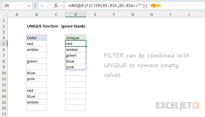
Working from the inside out, FILTER removes blank cells using the criterion <>"" (not equal to empty string). The filtered array is then passed to UNIQUE, which extracts the 5 unique colors.

For more details, see Unique values ignore blanks.

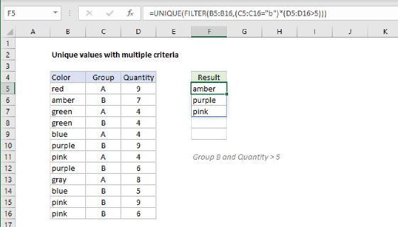
Unique values with criteria

To extract unique values that meet specific criteria, combine UNIQUE with FILTER. In the worksheet below, the goal is to extract unique colors for each group (A and B). The formula in E5 is:

=UNIQUE(FILTER(B5:B16,C5:C16=E4))

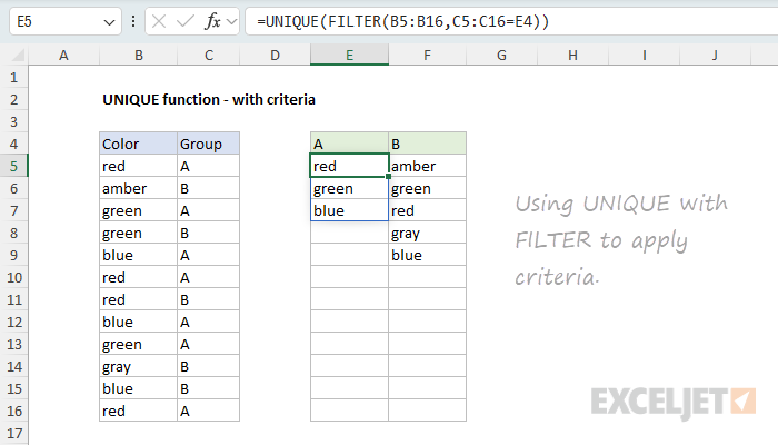
Working from the inside out, FILTER returns only colors where the corresponding group matches E4 ("A"). UNIQUE then extracts the unique colors from that filtered list. The formula in F5 works the same way, filtering for group "B" in F4.

For more details, see Unique values with criteria.

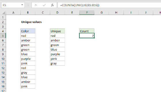
Count unique values

To count unique values, wrap UNIQUE with COUNTA or ROWS. In the worksheet below, the goal is to count the unique colors in B5:B16. The formula in F5 is:

=COUNTA(UNIQUE(B5:B16))

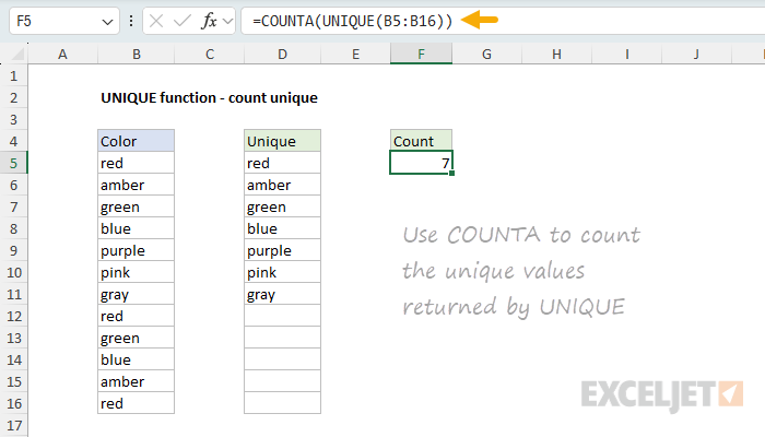
UNIQUE returns an array of 7 unique colors, which COUNTA counts. You can also use =ROWS(UNIQUE(B5:B16)) for the same result. If UNIQUE has already spilled results to the worksheet (as in D5), you can count them with a spill range reference:

=COUNTA(D5#)

The hash character (#) tells Excel to reference the entire spill range.

For more details, see Count unique values.

The GROUPBY function can also be used to count unique values. See GroupBy function.

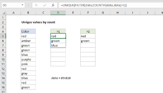
Unique values by count

To extract unique values that appear a certain number of times, combine UNIQUE with FILTER and COUNTIF. In the worksheet below, the goal is to extract colors that appear more than once (duplicates). The formula in D5 is:

=UNIQUE(FILTER(B5:B16,COUNTIF(B5:B16,B5:B16)>1))

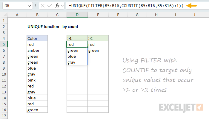
Working from the inside out, COUNTIF counts how many times each value appears in the data. The expression COUNTIF(data,data)>1 returns TRUE for values that appear more than once. FILTER keeps only those values, and UNIQUE extracts the unique ones. The result shows the 4 colors that appear more than once: red, green, blue, and gray. In cell E5, the formula has been adjusted to extract unique values that appear more than twice:

=UNIQUE(FILTER(B5:B16,COUNTIF(B5:B16,B5:B16)>2))

For more details, see Unique values by count.

Unique with non-adjacent columns

UNIQUE only works with adjacent columns. To extract unique values from non-adjacent columns, use FILTER or CHOOSECOLS to select the columns first. In the worksheet below, the goal is to extract unique combinations of Color (column B) and Region (column D), skipping Qty (column C). The formula in F5 is:

=SORT(UNIQUE(FILTER(B5:D15,{1,0,1})))

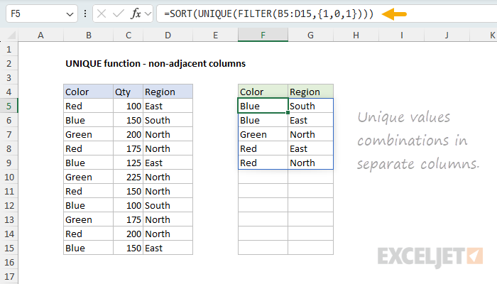
The array constant {1,0,1} tells FILTER to include the first and third columns while excluding the middle column. UNIQUE then extracts unique rows from the two remaining columns, and SORT arranges the results alphabetically. As an alternative, you can use the CHOOSECOLS function instead of an array constant like this:

=SORT(UNIQUE(CHOOSECOLS(B5:D15,1,3)))

For more details, see UNIQUE with non-adjacent columns.

Notes

• UNIQUE is case-insensitive. "APPLE", "Apple", and "apple" are treated as identical.
• UNIQUE treats text and numbers as different types. The text "10" and the number 10 are considered different values.
• Empty cells appear as zeros (0) in results. Use FILTER to exclude blanks before UNIQUE runs.
• The empty string "" and truly empty cells may be treated differently. Use <>"" to filter both.
• UNIQUE returns #SPILL! if the destination range isn't empty or doesn't have room for results.
• Cross-workbook references require both workbooks to be open. Closed workbooks return #REF!.
• UNIQUE won't automatically adjust the source range if data is added or deleted. Use an Excel Table or dynamic range if needed.