Summary
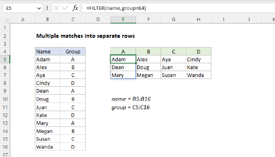
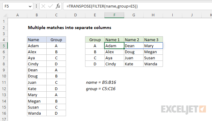
To extract multiple matches into separate columns based on a common value, you can use the FILTER function with the TRANSPOSE function. In the worksheet shown, the formula in cell F5 is:
=TRANSPOSE(FILTER(name,group=E5))
Where name (B5:B16) and group (C5:C16) are named ranges. The group names in E5:E8 and the name headings in F4:H4 are also created with formulas, as explained below. The explanation below covers two approaches (1) a modern approach based on the FILTER function and (2) a legacy approach based on INDEX and SMALL for older versions of Excel without the FILTER function.
Generic formula
=TRANSPOSE(FILTER(range1,range2=A1))
Explanation
In this example, the goal is to get all names in a given group into the same row, in separate columns, as seen in the worksheet. This is sometimes referred to as a "pivot" operation. The idea is to restructure the data into multiple columns using common values, which in this case are the group names. The explanation below includes two options: (1) a modern approach based on the FILTER function and (2) a legacy approach based on INDEX and SMALL for older versions of Excel without the FILTER function.
Modern approach
Several new functions in the current version of Excel make this task easier. First, to build a list of groups in alphabetical order, we use the UNIQUE function with the SORT function in cell E5 like this
=SORT(UNIQUE(group)) // returns {"A";"B";"C";"D"}
This formula spills the four unique group names into the range E5:E8. To generate the headings that appear in the range F4:H4, we use the SEQUENCE function with MAX and COUNTIF like this:
="Name "&SEQUENCE(1,MAX(COUNTIF(group,group)))
The COUNTIF function returns an array of counts for each group, and the MAX function returns the maximum count, which is 3. We use COUNTIF and MAX like this so that the header will automatically expand as needed when a group contains more names. The result is delivered to the SEQUENCE function as the columns argument, and SEQUENCE returns the array {1,2,3}:
SEQUENCE(1,3) // returns {1,2,3}
The result from SEQUENCE is then concatenated to the text string "Name ". The result is an array like this:
{"Name 1","Name 2","Name 3"}
We now have what we need to retrieve the names in each group. For this step, we use a formula like this in cell F5:
=TRANSPOSE(FILTER(name,group=E5))
Working from the inside out, the FILTER function retrieves the names in B5:B16 where the group = "A" (the value in E5), and TRANSPOSE converts the vertical array from FILTER into a horizontal array that spills into the range F5:H5. As the formula is copied down column F, the reference to E5 is relative and changes at each new row. As a final result, we have all names in each group together in the same row.
Note: It would be nice to use a reference to the spill range in E5:E8 (E5#) inside the FILTER function. However, Excel formulas won't currently return an array-of-arrays so this won't work.
Legacy solution
In older versions of Excel that don't offer the FILTER function, you can use a more complex array formula based on the INDEX function and the SMALL function to get multiple matches into separate columns. Enter the formula below in cell F5, then drag it down and across to fill in the other cells in the range F5:H8:
{=IFERROR(INDEX(name,SMALL(IF(group=$E5,ROW(name)-MIN(ROW(name))+1),COLUMNS($E$5:E5))),"")}
Note: This is an array formula and must be entered with Control + Shift + Enter in older versions of Excel.
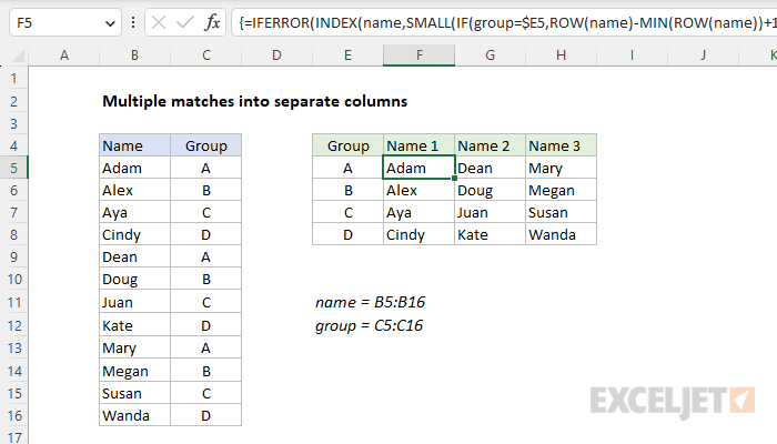
The gist of this formula is this: we are using the SMALL function to generate a row number corresponding to an "nth match" for each name in a group. Once we have the row number, we simply pass it into the INDEX function, which returns the value at that row. The trick is that SMALL is working with an array that is already filtered by group. The filtering is done with the IF function in this part of the formula:
IF(group=$E5,ROW(name)-MIN(ROW(name))+1)
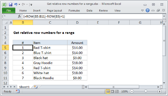
At a high level, this code gets the row numbers of all names that belong to a given group. It does this by testing the group in cell E5 against all values in the named range group. When the result is TRUE, the IF function returns the row number. The relative row numbers for all values in the data are created with the formula below:
ROW(name)-MIN(ROW(name))+1
See this page for details. The final result is an array that contains numbers where there is a match, and FALSE where not:
{1;FALSE;FALSE;FALSE;5;FALSE;FALSE;FALSE;9;FALSE;FALSE;FALSE}
As you can see, the only row numbers that survive the trip are those that correspond to the group in cell E5. This array goes into SMALL as the array argument. The value for k is created with an expanding range and the COLUMNS function:
COLUMNS($E$5:E5) // value for k
As the formula is copied across the table, the range expands, causing k to increment. The result is that the SMALL function returns the row number for each name in a given group. This number is supplied to the INDEX function as row_num, with the named range name as the array. Finally, INDEX returns the name associated with each row number.
Handling errors
When COLUMNS returns a value for k that does not exist, SMALL throws a #NUM error. This happens after all names for a given group have been extracted. To suppress this error, we wrap the formula in the IFERROR function and return an empty string ("").