=VLOOKUP(lookup_value, table_array, column_index_num, [range_lookup])- lookup_value - The value to look for in the first column of a table.
- table_array - The table from which to retrieve a value.
- column_index_num - The column in the table from which to retrieve a value.
- range_lookup - [optional] TRUE = approximate match (default). FALSE = exact match.
Using the VLOOKUP function
The Excel VLOOKUP function scans the first column in a table, finds a match, and returns a result from the same row. If VLOOKUP can't find a match, it returns a #N/A error or an "approximate match", depending on how it is configured. Because VLOOKUP is easy to use and has been in Excel for decades, it is the most popular function in Excel for basic lookups. You will find it in all kinds of worksheets in almost any business or industry. Although VLOOKUP is simple to configure, it has some default behaviors that can be dangerous in certain situations.
Key features
- Looks up values in the first column of a vertical table
- Returns data from any column to the right of the lookup column
- Supports exact match and approximate match modes
- Approximate match is the default (dangerous if exact match expected)
- Supports wildcards (* ?) for partial matching (exact match mode only)
- Is not case-sensitive
- Returns first match if duplicates exist
- Works in all versions of Excel
Table of contents
- VLOOKUP works with vertical data
- VLOOKUP uses column numbers
- VLOOKUP only looks right
- VLOOKUP has 2 matching modes
- VLOOKUP exact match example
- VLOOKUP approximate match example
- VLOOKUP has dangerous defaults
- VLOOKUP returns the first match
- VLOOKUP with a wildcard match
- VLOOKUP with a two-way lookup
- VLOOKUP with multiple criteria
- Handling VLOOKUP #N/A errors
- VLOOKUP performance tips
- More about VLOOKUP
Important: VLOOKUP performs an approximate match by default. See below for details.
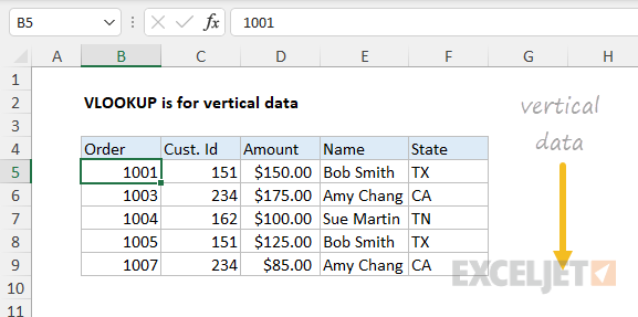
VLOOKUP works with vertical data
The "V" in VLOOKUP is for "Vertical". The purpose of VLOOKUP is to look up and retrieve information in a table organized vertically:
For example, with the table above, you can use VLOOKUP to find the amount for a given order like this:
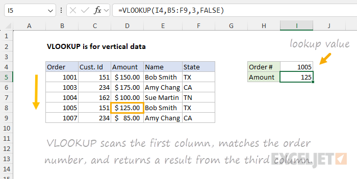
With the order number 1005 as a lookup value in cell I4, the result is 125. VLOOKUP scans the first column of the table, matches order number 1005, and returns 125, the amount. The formula in cell I5 is:
=VLOOKUP(I4,B5:F9,3,FALSE)
For now, just pay attention to these things:
- The lookup value is provided as I4. If this value is changed, VLOOKUP will return a new result.
- The lookup table is provided as the range B5:F9, which is the entire table.
- The lookup values (order numbers) are in the first column of the table.
- The result values (order amounts) are in the third column of the table.
- The column index number is given as 3.
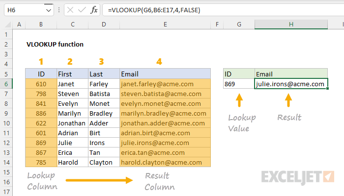
VLOOKUP uses column numbers
The VLOOKUP function uses column numbers to indicate the column from which a value should be retrieved. When you use VLOOKUP, imagine that every column in the table is numbered, starting at 1:
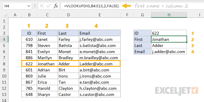
To retrieve a value from a given column, just provide the number for column_index_num. For example, to retrieve the first name in cell H4, we use 2 for column_index_num, as seen above. By changing only the column number, we can retrieve the first name, last name, and email address by asking for columns 2, 3, and 4:
=VLOOKUP(H3,B4:E13,2,FALSE) // first name
=VLOOKUP(H3,B4:E13,3,FALSE) // last name
=VLOOKUP(H3,B4:E13,4,FALSE) // email address
Notice that the only difference in the formulas above is the column number.
To see a short demo, watch this 3-minute video: How to use VLOOKUP
VLOOKUP only looks right
VLOOKUP can only look to the right. In other words, you can only retrieve data to the right of the first column in the table provided to VLOOKUP. For example, to look up information by ID in the table below, we must provide the range D3:F9 as the table, and that means we can only look up Email and Department:
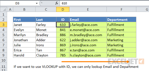
This is a fundamental limitation of VLOOKUP — the first column of the table must contain lookup values, and VLOOKUP can only access columns to the right. To retrieve information to the left (or right) of a lookup column, you can use the XLOOKUP function or an INDEX and MATCH formula.
VLOOKUP has 2 matching modes
VLOOKUP has two match modes: exact match and approximate match. The last argument, called range_lookup, controls which match mode is used. The word "range" in this case refers to "range of values" – when range_lookup is TRUE, VLOOKUP will match a range of values rather than an exact value. When range_lookup is FALSE, VLOOKUP will only allow an exact match:
=VLOOKUP(value,table,col_index,TRUE) // approximate match
=VLOOKUP(value,table,col_index,FALSE) // exact match
Pro tip: You can also supply zero (0) for an exact match, and 1 for an approximate match. Excel will evaluate 0 as FALSE and 1 as TRUE, so 0 and 1 are more compact equivalents.
VLOOKUP exact match example
In most cases, you'll probably want to use VLOOKUP in exact match mode. This makes sense when you have a unique key to use as a lookup value, for example, the movie title in this data:
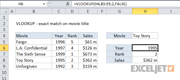
The formula in H6 to find Year, based on an exact match of the movie title, is:
=VLOOKUP(H4,B5:E9,2,FALSE) // FALSE = exact match
With "Toy Story" in H4, VLOOKUP finds a match in the fourth row in the table and returns 1995 as a result.
VLOOKUP approximate match example
In some cases, you will need an approximate match lookup instead of an exact match lookup. A good example is the problem of assigning a letter grade based on a score. In the worksheet below, we want to use the scores in column C to assign a grade using the table to the right in the range F5:G9, which is named "key". Here, we need to use VLOOKUP in approximate match mode, because in most cases, the exact score in column C will not be found in column F. The VLOOKUP formula in D5 is configured to perform an approximate match by setting the last argument to TRUE:
=VLOOKUP(C5,$G$5:$H$10,2,TRUE) // TRUE = approximate match
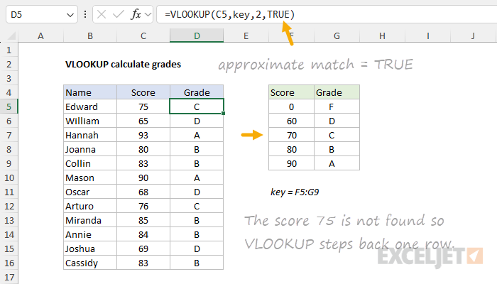
As the formula is copied down, VLOOKUP will scan values in column F looking for the score in column C. If an exact match is found, VLOOKUP will return the corresponding grade in that row. If an exact match is not found, VLOOKUP will stop at the first larger score, then "step back" and return the grade from the previous row.
Caution: for an approximate match, the table provided to VLOOKUP must be sorted in ascending order by the first column. If the table is not sorted, VLOOKUP may return incorrect or unexpected results, as explained in the next section.
Video: How to use VLOOKUP for approximate match
VLOOKUP has dangerous defaults
It is important to understand that VLOOKUP will perform an approximate match by default. This happens because range_lookup is optional and defaults to TRUE. This can cause big problems if you expect an exact match, as seen in the worksheet below. Here, the goal is to look up the amount for a given invoice number in cell F5. The formula in G5 is:
=VLOOKUP(F5,B5:D10,3) // approximate by default!
No value has been provided for range_lookup, so VLOOKUP performs an approximate match. Notice that invoice number 100235 does not exist in the data, but VLOOKUP returns 12,000. This happens because VLOOKUP scans the table until it reaches invoice 100236, then it "steps back" to invoice 100234 and returns the (incorrect) amount in that row:
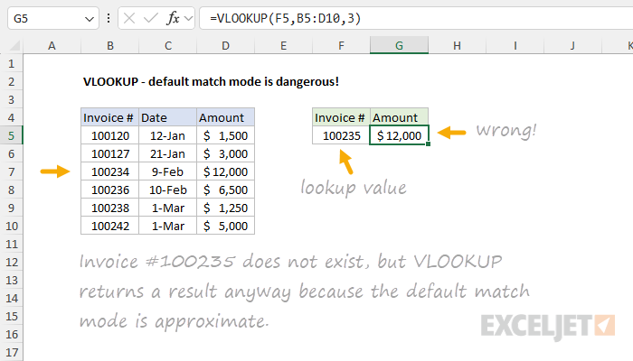
To fix this problem, enable exact matching by providing range_lookup as FALSE or 0:
=VLOOKUP(F5,B5:D10,3,FALSE) // exact match
This will cause VLOOKUP to return an #N/A error when an invoice number doesn't exist. If you like, you can use the IFNA function to return a more friendly result, as explained below.
The bottom line: If you don't supply a value for range_lookup, VLOOKUP will perform an approximate match. In this mode, VLOOKUP can return results that look fine but are in fact totally incorrect. For this reason, I recommend that you always set a value for range_lookup as a reminder of what you expect.
VLOOKUP returns the first match
If there is more than one matching value in a table, VLOOKUP will only find the first match. In the screen below, VLOOKUP is configured to get the price for the color "Green". There are three rows with the color Green, and VLOOKUP returns the price in the first row, which is $17.00. The formula in cell F5 is:
=VLOOKUP(E5,B5:C11,2,FALSE) // returns 17
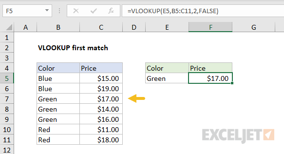
To retrieve the last match in a set of data, you can use the XLOOKUP function configured to perform a "reverse search". To retrieve all matches, use the FILTER function.
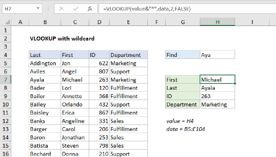
VLOOKUP with a wildcard match
The VLOOKUP function supports wildcards, which makes it possible to perform a partial match on a lookup value. To use wildcards with VLOOKUP, you must provide FALSE or zero (0) for range_lookup. In the screen below, the formula in H7 retrieves the first name, "Michael", after typing "Aya" into cell H4. Notice the asterisk (*) wildcard is concatenated to the lookup value inside the VLOOKUP formula:
=VLOOKUP($H$4&"*",$B$5:$E$104,2,FALSE)
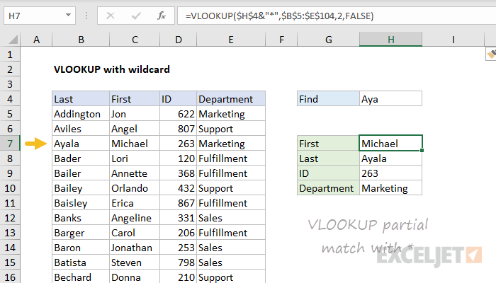
For a full explanation of this formula, see this example.
VLOOKUP with a two-way lookup
Inside the VLOOKUP function, column_index_num is normally hard-coded as a static number. However, you can create a dynamic column index by using the MATCH function to locate the desired column. This technique allows you to create a dynamic two-way lookup, matching on both rows and columns. In the screen below, VLOOKUP is configured to perform a lookup based on Name and Month like this:
=VLOOKUP(H4,B5:E13,MATCH(H5,B4:E4,0),0)
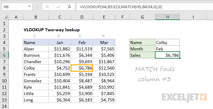
MATCH locates "Feb" in the range B4:E4 and returns 3 to VLOOKUP as the column number. For more details, see this example.
Note: In general, INDEX and MATCH is a more flexible way to perform two-way lookups.
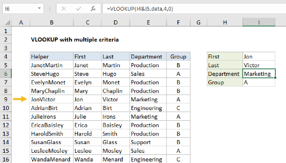
VLOOKUP with multiple criteria
The VLOOKUP function does not handle multiple criteria natively. However, you can use a helper column to join multiple fields together and use these fields as multiple criteria inside VLOOKUP. In the example below, Column B is a helper column that concatenates first and last names together with this formula:
=C5&D5 // helper column
VLOOKUP is configured to do the same thing to create a lookup value. The formula in H6 is:
=VLOOKUP(H4&H5,B5:E13,4,0)
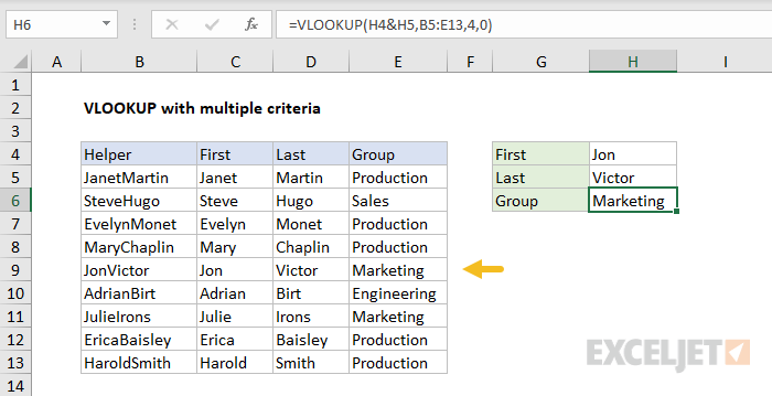
For details, see this example. For a more advanced, flexible approach, see this example.
Note: INDEX and MATCH and XLOOKUP are better for lookups based on multiple criteria.
Handling VLOOKUP #N/A errors
If you use VLOOKUP, you will inevitably run into the #N/A error. The #N/A error simply means "not found". For example, in the screen below, the lookup value "Toy Story 2" does not exist in the lookup table, and all three VLOOKUP formulas return #N/A:
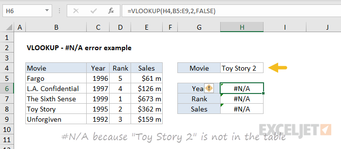
The #N/A error is useful because it tells you something is wrong. There are several reasons why VLOOKUP might return an #N/A error, including:
- The lookup value does not exist in the table
- The lookup value is misspelled or contains extra spaces
- Match mode is exact, but should be approximate
- The table range is not entered correctly
- The formula was copied, and the table reference is not locked
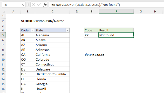
To "trap" the NA error and return a custom value, you can use the IFNA function like this:
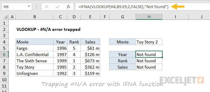
The formula in H6 is:
=IFNA(VLOOKUP(H4,B5:E9,2,FALSE),"Not found")
The message can be customized as desired. To return nothing (i.e., to display a blank result) when VLOOKUP returns #N/A you can use an empty string ("") like this:
=IFNA(VLOOKUP(H4,B5:E9,2,FALSE),"") // no message
You can also use the IFERROR function to trap VLOOKUP #N/A errors. However, use caution with IFERROR, because it will catch any error, not just the #N/A error. Read more: VLOOKUP without #N/A errors
VLOOKUP performance tips
VLOOKUP in exact match mode can be slow on large data sets. On the other hand, VLOOKUP in approximate match mode is very fast, but dangerous if you need an exact match because it might return an incorrect value. In a modern version of Excel, the easiest fix is to switch to a function like XLOOKUP, which has built-in support for a super-fast binary search. You could also use INDEX and XMATCH, since XMATCH also has the fast binary search option. If you are stuck in an older version of Excel without XLOOKUP or XMATCH, another option is to create a fast exact match formula by using VLOOKUP twice. This is a cool trick, but I wouldn't use this approach unless it is your only option. I would also avoid using full column references like A:A with VLOOKUP. Since an Excel workbook contains over 1 million rows, using full column references can cause major performance problems in certain cases by making Excel process millions of extra cells.
More about VLOOKUP
- VLOOKUP with multiple criteria (basic)
- VLOOKUP with multiple criteria (advanced)
- How to use VLOOKUP to merge tables
- 23 tips for using VLOOKUP
- XLOOKUP vs VLOOKUP
Notes
- VLOOKUP performs an approximate match by default.
- VLOOKUP is not case-sensitive.
- Range_lookup controls matching. FALSE = exact, TRUE = approximate (default).
- If range_lookup is omitted or TRUE:
- VLOOKUP will match the nearest value equal to or less than the lookup_value*.***
- Column 1 of table_array must be sorted in ascending order.
- If range_lookup is FALSE or zero for an exact match:
- VLOOKUP will perform an exact match.
- The table_array does not need to be sorted.