Explanation
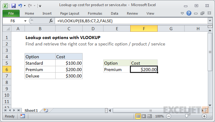
This is a basic example of VLOOKUP in "exact match" mode. The lookup value is B6, the table is the range B5:C7, the column is 2, and the last argument, FALSE, forces VLOOKUP to do an exact match. (Read why this is necessary here).
If VLOOKUP finds a matching value, the associated cost will be retrieved from the 2nd column (column C). If no match is found, VLOOKUP will return the #N/A error.
Related formulas
VLOOKUP without #N/A error
When VLOOKUP can't find a value in a lookup table, it returns the #N/A error. In this example, the goal is to remove the #N/A error that VLOOKUP returns when it can't find a lookup value. In general, the best way to do this is to use the IFNA function. However, the IFERROR function can also be used...
VLOOKUP from another workbook
In this example, the goal is to use VLOOKUP to find and retrieve price information for a given product stored in an external Excel workbook. The workbook exists in the same directory and the data in the file looks like this: Note the data itself is in the range B5:E13. VLOOKUP formula The formula...
VLOOKUP two-way lookup
In this example, the goal is to perform a two-way lookup based on the name in cell H4 and the month in cell H5 with the VLOOKUP function. Inside the VLOOKUP function, the column index argument is normally hard-coded as a static number. However, you can create a dynamic column index number by using...
VLOOKUP calculate grades
In this example, the goal is to calculate the correct grade for each name in column B using the score in column C and the table in F5:G9 as a "key" to assign grades. For convenience only, the range F5:G9 has been named key . This is a classic "approximate-match" lookup problem because it is not...
Get employee information with VLOOKUP
The goal is to look up and retrieve employee information in a table that contains unique id values in the first column. The VLOOKUP function is straightforward to use with data in this format, but you can easily use the XLOOKUP function as well. See below for a detailed explanation of both...
Merge tables with VLOOKUP
This is a standard "exact match" VLOOKUP formula with one exception: the column index is calculated using the COLUMN function. When the COLUMN function is used without any arguments, it returns a number that corresponds to the current column. In this case, the first instance of the formula in...
Related functions
VLOOKUP Function
The Excel VLOOKUP function is used to retrieve information from a table using a lookup value. The lookup values must appear in the first column of the table, and the information to retrieve is specified by column number. VLOOKUP supports approximate and exact...
Related videos
How to use VLOOKUP
VLOOKUP is one of the most important lookup functions in Excel. The V stands for "vertical" which means you can use VLOOKUP to look up values in a table that's arranged vertically. Let's take a look. Here we have a list of employees in a table. Let's use VLOOKUP to build a simple form that...
How to use VLOOKUP for approximate matches
In a lot of cases, you'll use VLOOKUP to find exact matches based on some kind of unique id, but there are many situations where you'll want to use VLOOKUP to find non-exact matches. A classic case is using VLOOKUP to find a commission rate based on a sales number. Let's take a look. Here we have...
How to replace nested IFs with VLOOKUP
You might build or inherit a worksheet that uses a series of nested IF statements to assign values of some kind. Many people use nested IF statements this way because the approach is easy once you get the hang of it. But nested IF statements can be difficult to maintain and debug. Let's look at how...
Why VLOOKUP is better than nested IFs
In this video we look at a few reasons why VLOOKUP is a better option than nested IF statements. In our last video, we used nested IF statements to calculate a commission rate based on a sales number. As a quick recap: The first formula is created with nested IF statements normally. The second...


