Summary
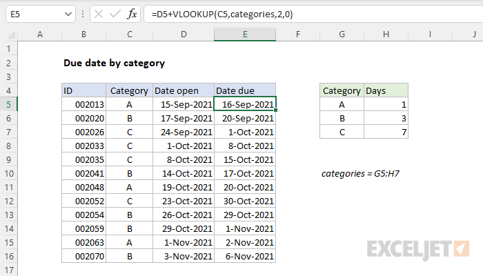
To calculate a due date based on category, where the category determines the due date, you can use a formula based on the VLOOKUP function. In the example shown, the formula in E5 is:
=D5+VLOOKUP(C5,categories,2,0)
Where categories is the named range G5:H7, the result is a due date in column E that is based on the category assigned in column C. This kind of formula can be used to set due dates, shipping dates, and other end dates where a group or category determines how much time is allotted.
Generic formula
=A1+VLOOKUP(category,table,column,0)
Explanation
In this example, the goal is to create a due date based on category, where each category has a different number of days allocated to complete a given task, issue, project, etc. The amount of time available to resolve each category is shown in column H, and categories is the named range G5:H7. The named range is for convenience and readability only. You can also use the absolute reference $G$5:$H$7.
Calculating days
The first task in this problem is to calculate the number of days to use for each category, as shown in the range G5:H7. One way to do it is to start adding IF statements like this:
=IF(C5="A",1,IF(C5="B",3,IF(C5="C",7)))
This approach is called "nested ifs". However, note how this tangles up the formula with the category data. If the days per category changes, the formula will need to be edited. If more categories are added, more IF functions will need to be added. This is not an ideal way to solve the problem.
A better approach is to use the VLOOKUP function to retrieve the number of days for a given category directly from G5:H7, which is named "categories" for convenience only. We can use VLOOKUP like this:
=VLOOKUP("A",categories,2,0) // returns 1
=VLOOKUP("B",categories,2,0) // returns 3
=VLOOKUP("C",categories,2,0) // returns 7
In the above formulas, the lookup_value is temporarily hardcoded as "A", "B", or "C". The table_array is provided as categories, which is the named range G5:H7 and column_index_num is 2, since we want days from the second column in. Finally, we use zero (0) for the range_lookup argument to force an exact match. To use this formula in the worksheet shown, we need to change lookup_value to C5:
=VLOOKUP(C5,categories,2,0)
Now, VLOOKUP will use the category shown in column C to retrieve the correct number of days from G5:H7. If the number of days for a category is changed, or if additional categories are added to the named range categories, the VLOOKUP will continue to return the correct result.
So far, so good. At this point, we have a number we can use for days, but we don't have a due date.
Creating a due date
The next task is to create the actual due date using the date given in column D. This is a simple problem, because dates in Excel are just serial numbers and can be added together like other numbers. To complete the formula, we only need to start with the date in D5, and add the VLOOKUP formula we created above:
=D5+VLOOKUP(C5,categories,2,0)
This formula gets the date from D5, retrieves the correct number of days for the category in C5 with VLOOKUP, and adds the two values together. The result in E5 is 16-Sep-2021, since we start with 15-Sep-2021 and add 1 day for category "A".
With XLOOKUP
For this problem, VLOOKUP works fine. However, you can also use the XLOOKUP function if you prefer like this:
=D5+XLOOKUP(C5,$G$5:$G$7,$H$5:$H$7)
Here we use absolute references since we can't use the named range categories directly for lookup_array and return_array. However, we can also get fancy and use the INDEX function with the named range like this:
=D5+XLOOKUP(C5,INDEX(categories,0,1),INDEX(categories,0,2))
Here we use zero for the row_num in INDEX, which causes INDEX to return the entire column.
Note: using an Excel Table instead of a named range for G5:H7 would be a good approach for XLOOKUP or VLOOKUP.
Workdays only
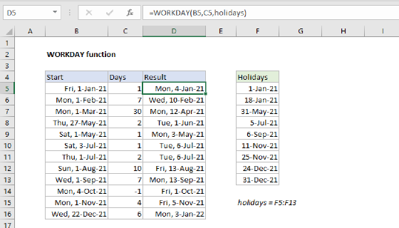
To create a due date based on workdays only you can alter the formula like this:
=WORKDAY(D5,VLOOKUP(C5,categories,2,0))
In this version, the WORKDAY function returns the final due date. The start date is the same and comes from column D. The VLOOKUP function is the same and returns days as before. The difference is that both values are returned directly to the WORKDAY function: D5 becomes the start_date and the result from VLOOKUP becomes the days argument.
WORKDAY uses the start date and days to create a date in the future, automatically ignoring Saturday and Sunday. WORKDAY can also ignore holidays as well, if they are provided as a range with valid dates. See the WORKDAY page for more information. If you need to customize the days treated as weekends, you can replace the WORKDAY function with the WORKDAY.INTL function, which offers more control over non-working days.
With hours
If you are using datetimes (i.e. date + time), you can adjust the categories table to show Excel hours (i.e. 8:00, 12:00, etc.) and use the same formula to determine a due date measured in hours. This works, because hours in Excel are fractional parts of 1 day. You will also need to change the number format used in column E to show date and time.