Summary
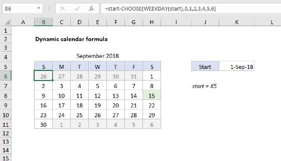
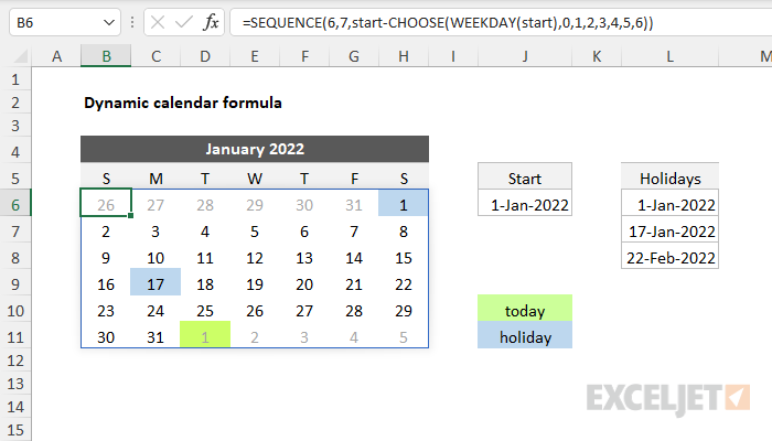
To create a dynamic monthly calendar with a formula, you can use the SEQUENCE function, with help from the CHOOSE and WEEKDAY functions. In the example shown, the formula in B6 is:
=SEQUENCE(6,7,start-CHOOSE(WEEKDAY(start),0,1,2,3,4,5,6))
where start is the named range J6. In the example shown, conditional formatting is used to highlight the current date and holidays, and lighten days in other months. See below for a full explanation.
Note: dynamic array functions are only available in Excel 365 and 2021. For a formula approach that works in older versions of Excel, see this example.
Explanation
Note: This example assumes the start date will be provided as the first of the month. See below for a formula that will automatically return the first day of the current month.
In this example, the goal is to generate a dynamic calendar for any given month, based on a start date entered in cell J6, which is named "start" We assume that start is a valid first-of-month date like 1-Jan-2022, 1-Feb-2022, 1-Mar-2022, etc. The final calendar should place each day of the month in a grid with each week starting on Sunday, as seen in the example. The solution explained below is based on the SEQUENCE function. SEQUENCE is one of the original dynamic array functions in Excel, and a perfect fit for this problem.
Background study
- Dynamic array formulas in Excel - overview
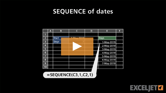
- The SEQUENCE function - 3 min video
- WEEKDAY function - overview and examples
- Custom number formats in Excel - overview
Short version
The explanation below is rather long. The short version is that the SEQUENCE function outputs a 6 x 7 array of 42 dates in a calendar grid, formatted to display the day only. This works because Excel dates are just serial numbers. The main challenge with this problem is figuring out what date to start with for a given month, which is always a Sunday. This is handled with the CHOOSE and WEEKDAY functions. Conditional formatting is used to highlight the current date and holidays and to lighten days in other months. Read below for all the details.
Basic SEQUENCE
The SEQUENCE function can be used to generate numeric sequences. For example, to generate the numbers 1 to 10 in ten rows, you can use SEQUENCE like this:
=SEQUENCE(10) // returns {1;2;3;4;5;6;7;8;9;10}
The result is an array that contains the numbers 1-10. The array spills into a vertical range of ten cells. SEQUENCE can generate arrays in rows and columns. For example, the following formula creates the numbers 1-10 in an array with 5 rows and 2 columns:
=SEQUENCE(5,2)
Similarly, the formula below will fill a 7 x 6 grid of cells with the numbers 1-42:
=SEQUENCE(6,7)
The screen below shows how these formulas behave on a worksheet:
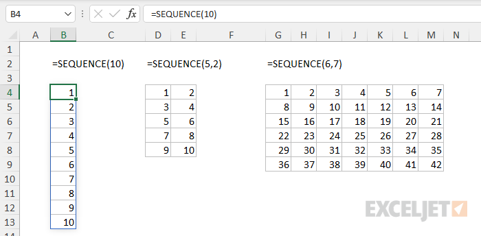
These are just numbers, not dates, but you can see the core concept.
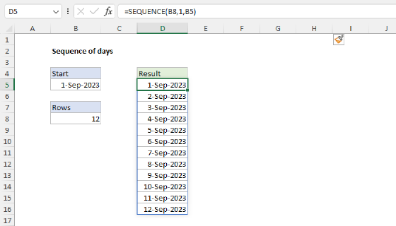
SEQUENCE with dates
Because Excel dates are just large serial numbers, the SEQUENCE function can easily be used to generate arrays of dates. For example, the formula below will generate dates for the 31 days of January 2022:
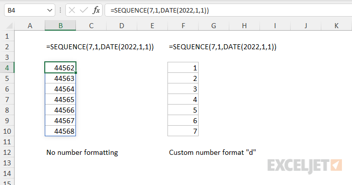
=SEQUENCE(7,1,DATE(2022,1,1))
Note: the DATE function is a safer way to hard code dates into formulas since dates entered as text can be misinterpreted.
To translate: we are asking for 7 numbers, in a 7 x 1 array, starting with January 1, 2022. SEQUENCE automatically defaults to a step value of 1, so the result is a list of serial numbers starting with 44562. We don't want to display serial numbers in our calendar, we want to show days. To do that we can use the custom number format "d". That will cause Excel to display just the day numbers. The screen below shows before and after:
Now let's see what happens if we ask for 6 x 7 grid, starting with January 1, 2022:
=SEQUENCE(6,7,DATE(2022,1,1))
Once we format the output with the custom number format "d", we see a total of 42 numbers, beginning with January 1. At the end of January, the month changes to February, and the day becomes 1 again:
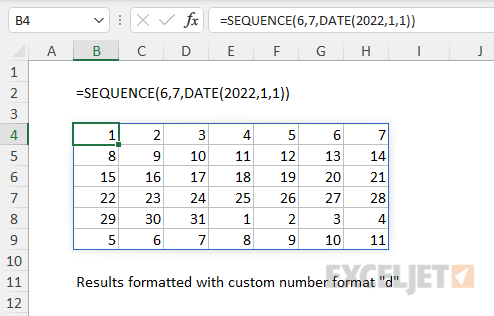
We still don't have a usable calendar, but we're getting closer!
To make a proper calendar, we need the first day in our grid to start on Sunday. If the first day of a month is not a Sunday, we need to start the grid on the last Sunday of the previous month. How can we calculate the last Sunday of the previous month? Before we get into specific functions, let's clarify the goal.
First Sunday
If the first of a month happens to be a Sunday, we're done. There's no need to do anything. The first of the month is our start date. However, if the first of the month is not a Sunday, we need to "roll back" some number of days to the prior Sunday. How many days do we need to roll back? This depends on what day of the week the first day of a month lands on. For example, if the first is a Tuesday, we need to roll back 2 days. If the first is a Friday, we need to roll back 5 days. And if the first is already a Sunday, we need to roll back 0 days.
Now we have a pretty good idea of what we need to do, we just need to implement that behavior in a formula. This is where the formula gets a bit tricky because we need to combine two functions, WEEKDAY and CHOOSE, in a way that most users won't recognize.
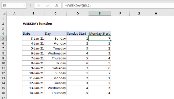
The WEEKDAY function
To figure out the day of the week, we use the WEEKDAY function. WEEKDAY returns a number for each day of the week. By default, WEEKDAY returns 1 for Sunday and 7 for Saturday. For example, WEEKDAY returns 7 for January 1, 2022, since the first is a Saturday:
=WEEKDAY(DATE(2022,1,1)) // returns 7
For January 2, 2022, WEEKDAY returns 1, since the second is a Sunday:
=WEEKDAY(DATE(2022,1,2)) // returns 1
To summarize, WEEKDAY will give us a number between 1-7 for each day of the week, and we can use that result to figure out how many days we need to roll back.
The CHOOSE function
The CHOOSE function is used to select arbitrary values by numeric position. For example, if we have the colors "red", "blue", and "green", we can use CHOOSE like this:
=CHOOSE(1,"red", "blue", "green") // returns "red"
=CHOOSE(2,"red", "blue", "green") // returns "blue"
=CHOOSE(3,"red", "blue", "green") // returns "green"
CHOOSE is a flexible function and accepts a list of text values, numbers, and cell references, in any combination.
CHOOSE + WEEKDAY
Next, we're going to combine CHOOSE and WEEKDAY to give us the correct "roll back" number like this:
=CHOOSE(WEEKDAY(start),0,1,2,3,4,5,6)
The index_num argument is provided by the WEEKDAY function. The other individual values given to CHOOSE are the rollback numbers, one for each day of the week. WEEKDAY returns a number between 1-7, and the CHOOSE function uses the number from WEEKDAY to select a number from the list of numbers provided. For example, if WEEKDAY returns 3 (Tuesday), CHOOSE returns 2:
CHOOSE(3,0,1,2,3,4,5,6) // returns 2
Now we are finally ready to use this rollback number to compute the first Sunday in the grid. Because dates are just numbers in Excel, the operation is simple – we just need to subtract the rollback number from the start date:
start-CHOOSE(WEEKDAY(start),0,1,2,3,4,5,6) // first Sunday
The result is a valid date that represents the first Sunday in the calendar grid.
Putting it all together
Now we need to combine the ideas explained above into a single formula based on the SEQUENCE function. We start off by asking for a 6 x 7 array of numbers like this:
=SEQUENCE(6,7 // 6 rows, 7 columns
Then, for the start argument, we simply provide the code we worked out above:
=SEQUENCE(6,7,start-CHOOSE(WEEKDAY(start),0,1,2,3,4,5,6))
The result is a full grid of 42 dates that can be displayed as a monthly calendar. If the start date in J6 is changed to another first-of-month date, the grid automatically updates.
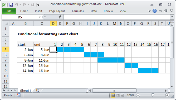
Conditional formatting rules
The conditional formatting rules to highlight the current date and holidays, and lighten days in other months are listed below:
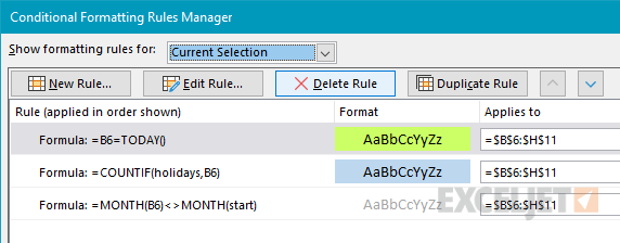
The formula for the current date is:
=B6=TODAY()
The formula to highlight holidays is based on the COUNTIF function:
=COUNTIF(holidays,B6)
If the count is anything but zero, the date must be a holiday. Holidays must be a range that contains valid Excel dates that represent non-working days. In the example shown, holidays is the named range L6:L8. You can add more holidays to this list as you like but don't forget to update the named range. Alternatively, you can define holidays as an Excel Table so the range updates automatically.
The formula to lighten days in other months is based on the MONTH function:
=MONTH(B6)<>MONTH(start)
If the month of the current date is different from the month of the date in J6, trigger the rule.
Read more: Conditional formatting with formulas, Excel custom number formats
Calendar Title
The formula to output the calendar title in cell B4 is based on the TEXT function:
=TEXT(start,"mmmm yyyy")
The title is centered over the calendar grid with the Center Across Selection. Select B4:H4, and use Control + 1 to open Format Cells, then select "Center Across Selection" from the Horizontal text alignment dropdown. This is a better option than merging cells since it doesn't alter the grid structure in the worksheet.
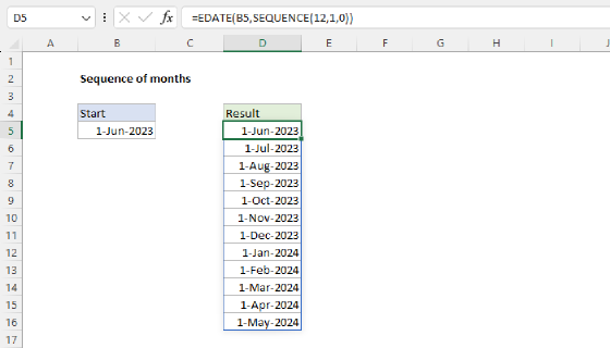
Perpetual calendar with current date
To create a perpetual calendar that updates automatically based on the current date, we need to update the formula to generate the first day of the current month on the fly. The first day of the current month can be calculated with the EOMONTH function like this:
=EOMONTH(TODAY(),-1)+1
You can use this formula directly in cell J6 and the calendar will always stay up to date. For an all-in-one formula, we can add the LET function like this:
=LET(start,EOMONTH(TODAY(),-1)+1,SEQUENCE(6,7,start-CHOOSE(WEEKDAY(start),0,1,2,3,4,5,6)))
Here, we use the LET function to define "start" as the first day of the current month, then run the original formula unchanged. The local variable "start" overrides the named range start on the worksheet, which can be deleted if desired.
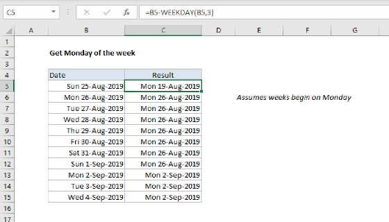
Monday start
To generate a calendar that starts on Monday instead of Sunday, you can use the following code inside of SEQUENCE as the start argument:
=start-CHOOSE(WEEKDAY(start),6,0,1,2,3,4,5)
Using the same logic explained above, this code rolls back the start date as needed to begin the calendar on Monday. This example has more information on rolling back dates to previous days of the week.