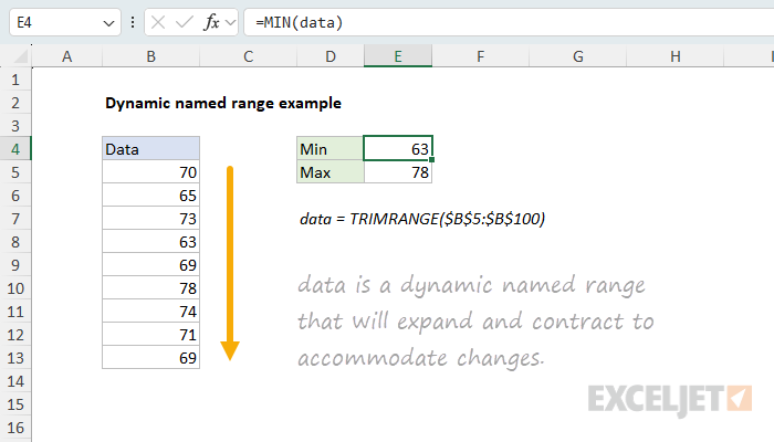
A dynamic named range, also called simply a "dynamic range" is a specially constructed range that expands automatically to accommodate new data. In the example shown, we have a small set of data in B5:B13, and two formulas calculating a minimum and maximum value like this:
=MAX(data)
=MIN(data)
Where "data" is a dynamic named range corresponding to B5:B13. In the example shown, the named range is defined with a formula based on the TRIMRANGE function:
=TRIMRANGE($B$5:$B$100)
TRIMRANGE is only available in Excel 365. In older versions of Excel, the same range can be created with a formula based on the OFFSET or INDEX functions, or with an Excel Table, as explained below.
The primary advantage of a dynamic named range is that the reference responds to changes. If values are removed from the bottom of the list, the range contracts. If values are added to the bottom of the list, the range expands. This minimizes the number of cells Excel needs to calculate and provides an easy-to-use reference that targets only data of interest.
Create a dynamic named range with TRIMRANGE
In Excel 365, the easiest way to create a dynamic named range is with the TRIMRANGE function. TRIMRANGE removes empty rows and columns from the outer edges of a range and returns a "trimmed" range that contains only data. To create the named range "data" in the example shown, open the Name Manager with the keyboard shortcut Control + F3, click New, enter the name "data", then enter a formula like this:
=TRIMRANGE($B$5:$B$100)
TRIMRANGE trims away the empty cells at the bottom of B5:B100 and returns B5:B13. If more values are added below the existing data, the range expands to include them. If values are removed from the bottom of the list, the range contracts. The formulas in E4 and E5 then return the minimum and maximum values in the trimmed range:
=MIN(data)
=MAX(data)
You can also trim a range with the dot operator, a compact syntax added to Excel at the same time as TRIMRANGE. A dot after the colon trims trailing empty rows and columns, so the formula below is equivalent to the TRIMRANGE formula above:
=$B$5:.$B$100
Both forms do the same thing, so use whichever you find easier to read. Note that references in a named range should be absolute so that the name works the same from any cell in the workbook. Excel will add the sheet name and absolute references automatically if you select the range by clicking on the worksheet.
TRIMRANGE and the dot operator are only available in Excel 365. For older versions of Excel, use one of the approaches below.
Create a dynamic named range with OFFSET or INDEX
In versions of Excel without TRIMRANGE, the traditional approach is to define the named range with a formula based on the OFFSET or INDEX functions. For example, the named range in the example shown can also be defined with OFFSET like this:
=OFFSET($B$5,0,0,COUNTA($B$5:$B$100))
The links below provide details on how to do this:
Using a formula like this gives you exactly the range you want without any overhead, and works in all versions of Excel. However, formulas that define dynamic named ranges with OFFSET or INDEX can be difficult to understand.
Create a dynamic named range with an Excel Table
The other way to create a dynamic named range is to use an Excel Table. Excel Tables automatically change to fit data and provide a formula syntax called "structured references" that can be used to target table elements by name. See the links below for more information: