MONTH Function

The MONTH function extracts the month from a given date as a number between 1 and 12. For example, given the date "June 12, 2021", the MONTH function returns 6 for June. MONTH takes just one argument, serial_number, which must be a valid Excel date.

The MONTH function returns a number. If you need a month's name, use the TEXT function as shown below. The MONTH function "resets" every 12 months (like a calendar or clock). To work with month durations larger than 12, use a formula to calculate months between dates.

Key features

• Returns month as integer 1-12 (1=January, 12=December)
• Works with dates as text or Excel serial numbers
• Often combined with YEAR, DAY, and DATE for date manipulation
• Returns a number, not a month name

Table of contents

• Basic usage
• Get month from date
• Get month name from date
• Get quarter from date
• Get last day of month
• Sum by month ignore year
• Count birthdays by month
• Filter by month
• Related functions
• Notes

Basic usage

MONTH takes just one argument, which must be a valid date or a text value that Excel can convert into a date. With the date March 15, 2026 in cell A1, all of these formulas will return 3:

=MONTH(A1) // returns 3
=MONTH("15-Mar-2026") // returns 3
=MONTH(DATE(2026,3,15)) // returns 3

Dates can be supplied to the MONTH function as text (e.g., "13-Aug-2021") or as native Excel dates, which are large serial numbers. To create a date value from scratch with separate year, month, and day inputs, use the DATE function.

Get month from date

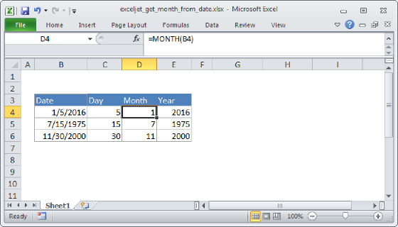
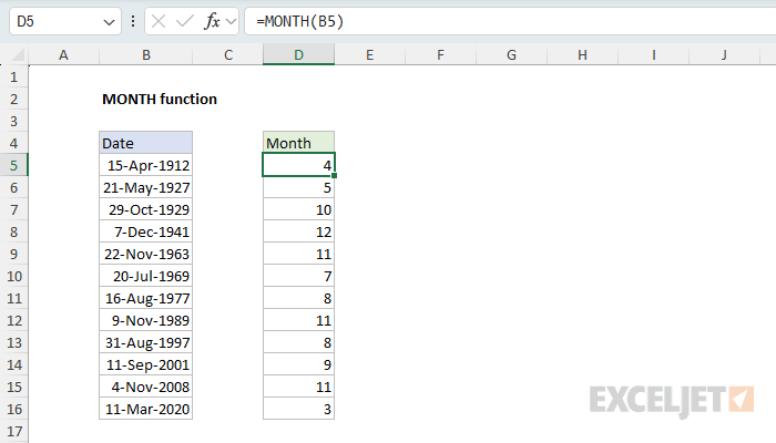
In the worksheet below, the goal is to extract the month number from dates. The formula in C5 is:

=MONTH(B5)

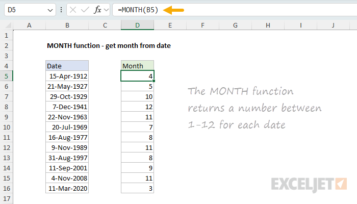
The MONTH function takes just one argument, the date from which to extract the month. In this example, with the date April 15, 1912 in cell B5, MONTH returns 4 for April. As the formula is copied down, it returns the month for each date in column B.

You can use MONTH to extract the month from a date entered as text (e.g., =MONTH("1/5/2016")), but using text for dates can produce unpredictable results on computers using different regional date settings. It's better to supply a cell reference that contains a valid date.

For more details, see Get month from date.

Get month name from date

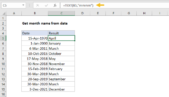
One thing that confuses new users to Excel is how to get the month name with the MONTH function. Short answer: you can't. The MONTH function returns a number, not a month name. You could use a more complicated formula to perform a lookup, but there is no need. The simplest way to get a month name from a date is to use the TEXT function. In the worksheet below, the goal is to extract the full month name from dates in column B. The formula in C5 is:

=TEXT(B5,"mmmm")

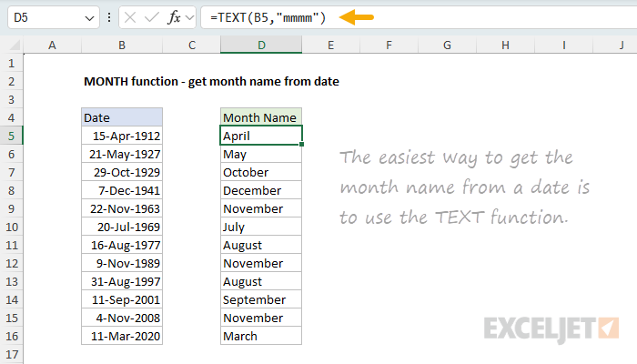
The TEXT function converts values to text using the number format you provide. The format "mmmm" returns the full month name (e.g., "January"), while "mmm" returns an abbreviated name (e.g., "Jan"). Note that the date is lost in the conversion — only the text for the month name remains.

Tip: If you only need to display a month name without converting to text, apply a custom number format directly to the cell containing the date.

For more details, see Get month name from date.

Get quarter from date

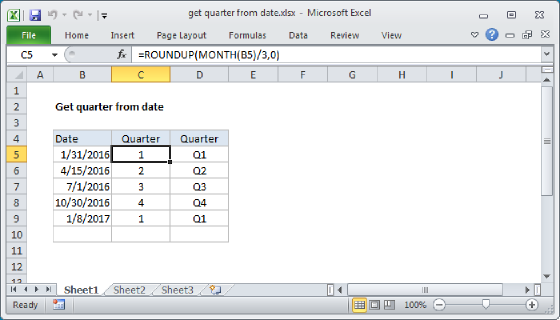
The MONTH function can be combined with the ROUNDUP function to calculate the quarter (1, 2, 3, or 4) for any date. In the worksheet below, the goal is to return the quarter number for dates in column B. The formula in C5 is:

=ROUNDUP(MONTH(B5)/3,0)

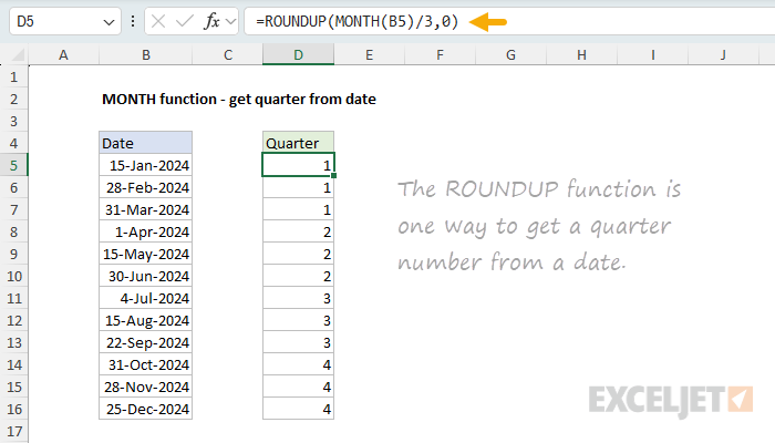
This formula works by dividing the month number by 3, then rounding up to the nearest integer. For example, January is month 1, and 1/3 = 0.33, which rounds up to 1 (Q1). June is month 6, and 6/3 = 2, which is already a whole number (Q2). To include "Q" in the result, concatenate it to the formula:

="Q"&ROUNDUP(MONTH(B5)/3,0)

For more details, see Get quarter from date.

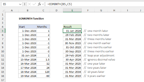
Get last day of month

The easiest way to get the last day of a month is with the EOMONTH function. However, you can also use MONTH with DATE to achieve the same result. In the worksheet below, the goal is to return the last day of the month for dates in column B. The formula in C5 is:

=DATE(YEAR(B5),MONTH(B5)+1,0)

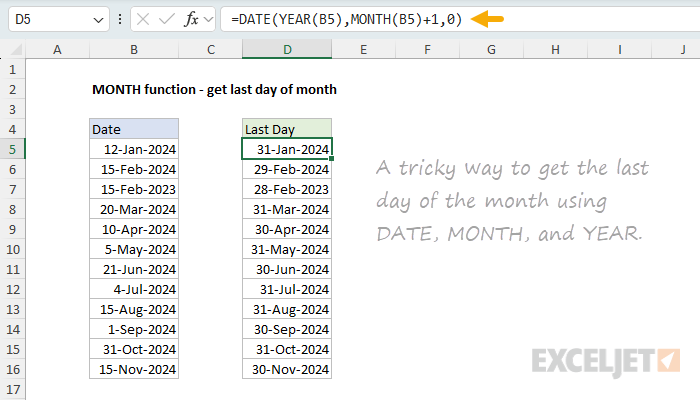
This formula works by using the DATE function with day set to zero. When you supply 0 as the day argument, DATE "rolls back" one day to the last day of the previous month. So, by adding 1 to the month and using 0 for day, DATE returns the last day of the original month.

Note: the EOMONTH function provides a more direct way to solve this problem: =EOMONTH(B5,0), but I include the DATE formula above because it shows that using a day value of 0 can be used to get the last day of the previous month.

For more details, see Get last day of month.

Sum by month ignore year

The MONTH function is useful for summarizing data by month while ignoring year values. In the worksheet below, the goal is to sum amounts by month across multiple years. The formula in F5 is:

=SUMPRODUCT((MONTH($B$5:$B$16)=MONTH(E5&1))*$C$5:$C$16)

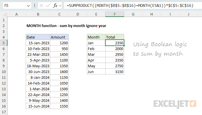
This formula uses the SUMPRODUCT function with MONTH to test each date against a target month number. The expression MONTH(E5&1) is a tricky way to convert the month name in E5 (e.g., "Jan") to a month number by concatenating "1" to create a text string like "Jan1", which Excel interprets as a date. See more details here.

When MONTH extracts the month from each date in the range and compares it to the target month, the result is an array of TRUE/FALSE values. Multiplying by the amounts converts TRUE to 1 and FALSE to 0, effectively summing only amounts where the month matches. This is an example using Boolean logic in an array formula to cancel out the amounts for months that don't match.

For more details, see Sum by month ignore year.

Note: In Excel 2021 and later, you can use the SUM function instead of the SUMPRODUCT function. However, SUMPRODUCT is a good solution because it works in all versions of Excel. For more information, see Why SUMPRODUCT?

Count birthdays by month

The MONTH function can also be used to count dates by month. This is handy for counting birthdays by month. In the worksheet below, the goal is to count how many birthdays fall in each month shown in column E. The formula in F5 is:

=SUMPRODUCT(--(MONTH($C$5:$C$16)=MONTH(E5&1)))

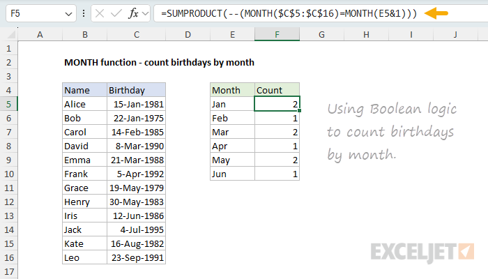
Like the sum-by-month example above, this formula uses Boolean logic in an array formula to cancel out the counts for months that don't match. It also uses the same trick to convert the month name in E5 (e.g., "Jan") to a month number before comparing it to the target month. MONTH extracts the month number from each birthday, and the result is compared to the target month. The result is an array of TRUE/FALSE values. The double negative (--) converts the TRUE/FALSE values to 1s and 0s, and SUMPRODUCT sums the result to give a count.

Note: COUNTIF won't work for this problem because it only accepts ranges, not arrays from expressions like =MONTH(range).

For more details, see Count birthdays by month.

Filter by month

You can use the FILTER function with MONTH to extract rows that match a specific month. In the worksheet below, the goal is to filter the data to show only rows from July (month 7 in cell H2). The formula in F5 is:

=FILTER(B5:D15,MONTH(C5:C15)=H2,"No data")

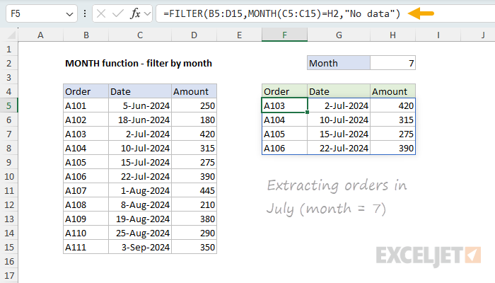
Here, MONTH(C5:C15)=H2 creates an array of TRUE/FALSE values: TRUE for dates in July, FALSE for all others. The FILTER function uses this array to filter the data range, and only rows where the result is TRUE appear in the output. The if_empty argument is set to "No data" in case no matching data is found.

To filter by both month and year, use Boolean logic:

=FILTER(B5:D15,(MONTH(C5:C15)=H2)*(YEAR(C5:C15)=2024),"No data")

For more details, see Filter by date.

Notes

• MONTH returns #VALUE! if the date is not recognized.
• MONTH returns #NUM! if a date is out of range (e.g., -1).
• Text dates can cause problems. Use cell references to valid dates when possible.