Date is same month and year

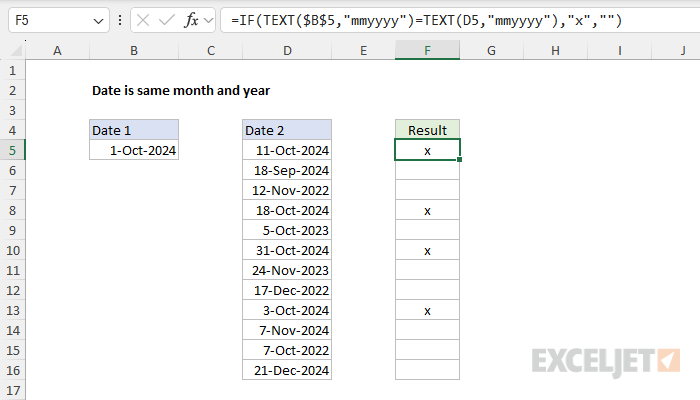
In this example, the goal is to mark dates in column D with an "x" when they have the same year and month as the date in cell B5. We don't care at all about the day. At a high level, we can easily use the IF function to return "x" for qualifying dates, so the challenge is in creating a logical test we can use inside IF that will properly test the dates. We want this test to return TRUE when two dates are in the same month and year and FALSE if not.

This problem is an interesting example of how a longer formula can be shortened to a simpler formula by paying attention to how the formula works and looking for ways to accomplish the same thing with less code. This article explains three ways to solve this problem: (1) a classic long-form formula, (2) a medium-form alternative, and (3) the compact short-form formula above.

Long-form with AND, YEAR, and MONTH

The classic long-form solution breaks each date into parts and uses a combination of the AND, YEAR, and MONTH functions to perform a logical test. We start with the logic we need: "Given two dates, if the year is the same, and if the month is the same, the result should be TRUE". We can translate this logic into an Excel formula like this:

=AND(YEAR($B$5)=YEAR(D5),MONTH($B$5)=MONTH(D5))

The literal translation for this formula is: If the year in B5 is equal to the year in D5 AND if the month in B5 is equal to the month in D5, return TRUE. Otherwise, return FALSE. Notice that cell B5 is an absolute reference to prevent it from changing as the formula is copied down the column. With 1-Oct-2024 in cell B5 and 11-Oct-2024 in cell D5, the formula evaluates like this:

=AND(YEAR($B$5)=YEAR(D5),MONTH($B$5)=MONTH(D5))
=AND(2024=2024,10=10)
=AND(TRUE,TRUE)
=TRUE

However, on the next row, where cell D6 contains the date 18-Sep-2024, the formula will evaluate like this:

=AND(YEAR($B$5)=YEAR(D6),MONTH($B$5)=MONTH(D6))
=AND(2024=2024,10=9)
=AND(TRUE,FALSE)
=FALSE

The last step is to include the logical test above in a formula that will mark dates that pass the test with an "x". We can easily do that with the IF function like this:

=IF(AND(YEAR($B$5)=YEAR(D5),MONTH($B$5)=MONTH(D5)),"x","")

As the formula is copied down, $B$5 is an absolute reference and does not change, while D5 is relative and changes at each new row. The result is that each date in column D is tested against the date in cell B5. When the test returns TRUE, the IF function returns "x". When the test returns FALSE, IF returns an empty string (""). This formula does the job and works fine. However, with a bit of creativity, we can streamline things quite a lot.

Medium-form with YEAR, MONTH, and concatenation

In the previous long-form formula, our logical test looks like this:

=AND(YEAR($B$5)=YEAR(D5),MONTH($B$5)=MONTH(D5))

Notice we are using many function calls for a fairly simple problem. Let's see what we can do to shorten things up a bit. If you look at the code, you can see we are extracting the year and month from each date and comparing each pair separately. Then, we use AND to evaluate the two results. Can we compare year and month in one step and eliminate AND? Yes. One way to do it is to join the month and year for each date together and then test the two strings in one step like this:

=MONTH($B$5)&YEAR($B$5)=MONTH(D5)&YEAR(D5)

This is a small improvement, but it is significant. We've reorganized the functions because we want the year and month for each date together. Because we are testing the year and month in one step, we no longer need the AND function. We combine the values with concatenation using the ampersand (&), creating a text string. For the date in D5, the code above evaluates like this:

=MONTH($B$5)&YEAR($B$5)=MONTH(D5)&YEAR(D5)
=10&2024=10&2024
="102024"="102024"
=TRUE

It might seem strange to work with the month and year as a text string, but it creates a human-readable value that contains all the information we need. For example, for a date in October 2024, we'll end up with "102024". After we place this logic inside the IF function, the final medium-form formula looks like this:

=IF(MONTH($B$5)&YEAR($B$5)=MONTH(D5)&YEAR(D5),"x","")

As with the original solution, this formula will mark all dates in the same month and year with an "x". Can we take this idea further and streamline the formula even more? Yes.

Short-form with the TEXT function

In the medium-form formula, we've eliminated the AND function by concatenating the year and month for each date together. This gives us a simple text string for each date that we can compare, but we still need to call YEAR and MONTH twice, once for each date. The logical test looks like this:

=MONTH($B$5)&YEAR($B$5)=MONTH(D5)&YEAR(D5)

How can we take this idea further and make the formula shorter? The trick is to bring in the TEXT function, which can format numbers as text using a variety of special codes. The TEXT function returns a number formatted as text. The format itself is provided as an argument called format_text. Because dates are numbers, we can get a date in the form "mmyyyy" in one step like this:

=TEXT($B$5,"mmyyyy")

With 1-Oct-2024 in cell B5, TEXT returns the text string "102024", which is exactly what we got with the MONTH and YEAR function in the previous formula. This means we can remove YEAR and MONTH altogether and use only the TEXT function like this:

=TEXT($B$5,"mmyyyy")=TEXT(D5,"mmyyyy")

This formula evaluates the same way as before:

TEXT($B$5,"mmyyyy")=TEXT(D5,"mmyyyy")
="102024"="102024"
=TRUE

The final formula with the IF function added back in looks like this:

=IF(TEXT($B$5,"mmyyyy")=TEXT(D5,"mmyyyy"),"x","")

This is a significant improvement. We've reduced function calls by more than half. The reworked formula is more compact, easier to read, and easier to extend, due to the flexibility of the TEXT function.

Summary

This article explains three formulas to check if two dates share the same month and year, beginning with a traditional long-form solution and ending with a more elegant short-form solution based on the TEXT function. By switching from separate YEAR and MONTH function calls to TEXT with a date format like "mmyyyy", we were able to cut the total number of function calls in half:

1. Long-form (6 function calls): IF, AND, YEAR(2), and MONTH(2)
2. Medium form (5 function calls): IF, YEAR(2) and MONTH(2)
3. Short form (3 function calls): IF and TEXT(2)

Each method is a bit more compact and efficient than the previous one. This problem is a good example of how a better understanding of Excel's functions can lead to simpler, more elegant formulas. It's also a great demonstration of the versatility of the TEXT function.