Summary
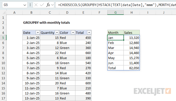
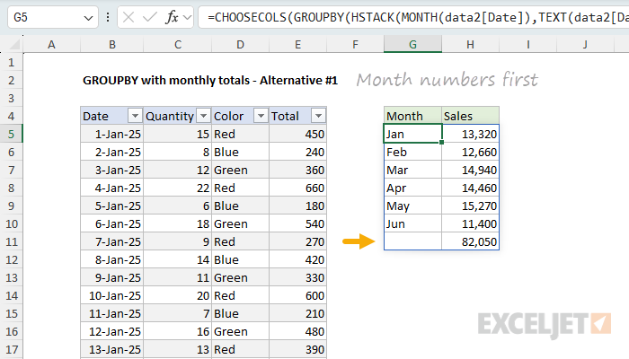
To generate monthly totals using the GROUPBY function, you can use a formula that integrates several functions in Excel, including GROUPBY, CHOOSECOLS, HSTACK, TEXT, MONTH, and SUM. In the worksheet shown, the formula in cell G5 is:
=CHOOSECOLS(GROUPBY(HSTACK(TEXT(data[Date],"mmm"),MONTH(data[Date])),data[Total],SUM,,,2,,1),{1,3})
The source data is in an Excel Table named data in the range B4:E179, which contains daily sales data for the first 6 months of 2025. The result is a total for each month in columns G and H. This is a fully dynamic solution. If the source data in the table changes, the monthly totals will recalculate as needed.
After I published this article, I got an email from a reader suggesting what I think is an even better approach. The core idea is to leave all of the dates as dates, but to remap them to the first day of each month, then group. See details below under Formula Alternative #2.
Explanation
In this example, the goal is to generate monthly totals using the GROUPBY function. This is a tricky problem in Excel because typically, source data contains a regular date field and not a separate field with month names. In addition, the GROUPBY function will, by default, sort everything in alphabetical order. This means when we add month names, they will sort A-Z and end up in the wrong order. Part of the challenge is figuring out the best way to sort the month names as part of the GROUPBY formula. To explain how this all works, let's build the solution step by step.
Table of contents
- Excel data for source data
- The core GROUPBY formula
- GROUPBY sort options
- Adding the month numbers to sort by
- Sorting the table by month number
- Removing the month numbers
- Summary of steps
- Alternative formula #1
- Alternative formula #2
- Formula for older versions of Excel
- Final thoughts
Excel data for source data
The source data is in an Excel Table named data in the range B4:E179, which contains daily sales data for the first 6 months of 2025. It's not necessary to use an Excel table to solve this problem, but it makes the formula a bit easier to read and understand. Plus, it means that the solution is dynamic - if the source data is added or removed, the monthly subtotals will recalculate as needed.
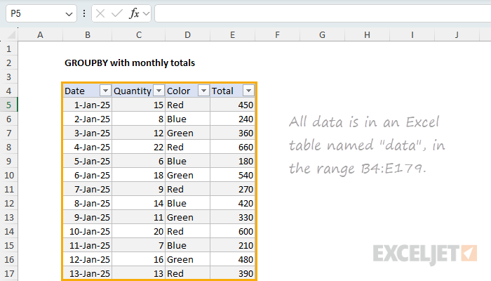
Note: The source data contains only the first 6 months of 2025. This is to keep the example simple. The solution will work with any number of months.
The core GROUPBY formula
The GROUPBY function excels at grouping data. In this example, we're going to use GROUPBY to group the data by month. The main challenge initially is that we don't have month names in the data. We only have the raw dates. This means we need to create our own month names in the formula. An easy way to do that is to use the TEXT function, which allows us to generate month names any way we like using Excel's custom number format codes. In this case, we will abbreviate the month names using the format code "mmm". For example, with a date like 12-Jan-2025 in cell A1, TEXT would return "Jan":
=TEXT("12-Jan-2025","mmm") // returns "Jan"
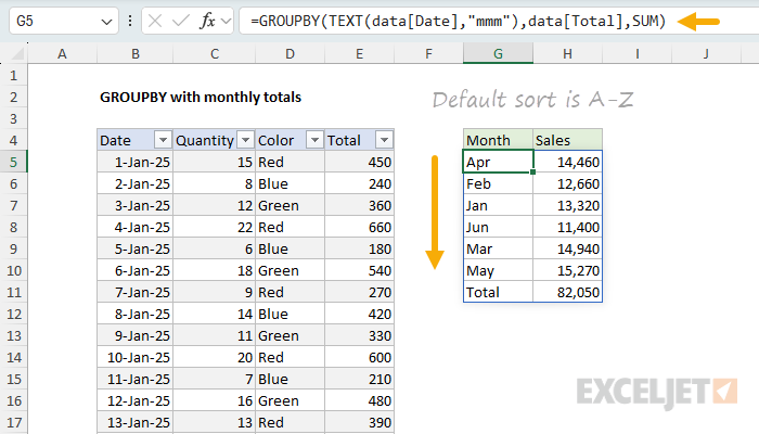
The complete formula in cell G5 below looks like this:
=GROUPBY(TEXT(data[Date],"mmm"),data[Total],SUM)
- The first argument to GROUPBY is the data to group. Here we use the TEXT function to create the month names as shown above, with the code
=TEXT(data[Date],"mmm"). The result is a new column of month names derived directly from the dates. This column doesn't actually exist in the source data, but we can use it as a row field in the GROUPBY function. - The second argument to GROUPBY is the data to aggregate. In this case, we want to aggregate the sales numbers in the Total column, so we use data[Total].
- The third argument to GROUPBY is the function to use to aggregate the data. Because we want total sales per month, we want to use the SUM function.
This formula works nicely. You can see that we get a clean breakdown by month for the first six months of 2025. However, there is a problem. Notice that the month names do not appear in chronological order. Instead, they are sorted alphabetically. This is because the GROUPBY function sorts grouped values in alphabetical order by default.
GROUPBY sort options
By default, the GROUPBY function will sort values in standard ascending (A-Z) order, beginning with the leftmost row field. The result is that the month names are sorted alphabetically, starting with "Apr". To override the default sort order, we can provide a value for the sort_order argument, which is given as an index number that can be positive (A-Z) or negative (Z-A). The number itself corresponds to the columns in the table, starting with 1 for the first column. For example, to sort the table by month name in descending (Z-A) order, we can provide -1 for sort_order in the GROUPBY function, like this:
=GROUPBY(TEXT(data[Date],"mmm"),data[Total],SUM,,,-1)
However, as you can see, that doesn't help. The month names are still sorted alphabetically, but in reverse order, so now the first month name is "May" instead of "Apr":
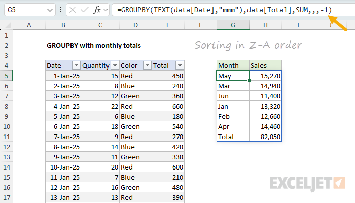
We'll need to use a different approach.
Adding the month numbers to sort by
To sort the month names in chronological order, we need a different approach. The core problem is that we only have the month names as text, but what we need to sort in chronological order are month numbers. To get the month numbers, we can use the MONTH function, which returns the month number for a given date. For example, with a date like 12-Mar-2025, MONTH would return 3:
=MONTH("12-Mar-2025") // returns 3
We can get month numbers for all dates in the source data like this:
=MONTH(data[Date]) // returns 1-12 for all dates
Because there are 175 dates in the source data, this MONTH returns an array of 175 month numbers. Like the month names, this column does not exist in the source data, but we can add it as a second row field using the HSTACK function. HSTACK stacks arrays horizontally, which lets us work around the limitation that GROUPBY only allows one row field. We can use it to add the month numbers as a second row field like this:
=GROUPBY(HSTACK(TEXT(data[Date],"mmm"),MONTH(data[Date])),data[Total],SUM)
As you can see, this adds the month numbers as a second row field. The first row field is the month name, and the second row field is the month number.
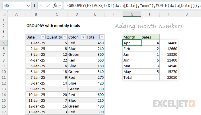
Notice I've also removed the sort order setting, so we are back to an alphabetical sort. The month numbers appear as a second row field, but the table is still being sorted by the left-most row field, which is the month name.
Note: We don't really want the month numbers in the table, and we'll get rid of them in a another step below.
Sorting the table by month number
We are now at the point where we can finally sort the table by month number. To do that, we need to specify the column to sort by as an index number. Because we've added a column, we need to sort by column 2, the month number. We can do that by adding a sort_order argument to the GROUPBY function like this:
=GROUPBY(HSTACK(TEXT(data[Date],"mmm"),MONTH(data[Date])),data[Total],SUM,,,2)
Unfortunately, this doesn't work. Why? The problem is that GROUPBY uses a hierarchical relationship between row fields by default. This means the month names override the month numbers, because they appear first in the table:
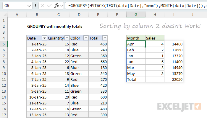
We need a way to unlink the month names from the month numbers for sorting. We can do that by supplying 1 for the last argument, which is called field_relationship. This tells GROUPBY to use a table relationship instead of a hierarchy relationship:
=GROUPBY(HSTACK(TEXT(data[Date],"mmm"),MONTH(data[Date])),data[Total],SUM,,,2,,1)
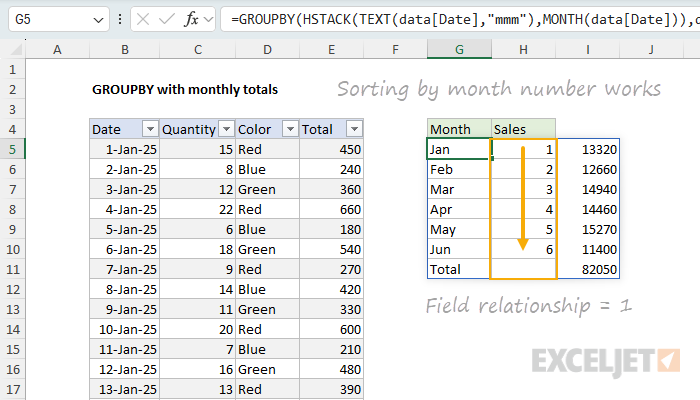
This works! The month names are no longer overriding the month numbers, and the table is sorted by month number.
Note: you might wonder about adding the month numbers as the first row field instead of the second. This also works. But one consequence is that the word "Total" will be removed from the table when we remove the month number column in the next step. In the end, I decided to keep the month numbers as the second row field because it makes a good example of how the field relationship argument works. See the Alternative formula section below for more details.
Removing the month numbers
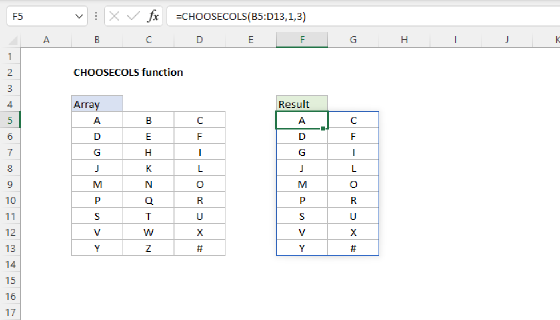
The last step in the problem is to remove the month numbers from the table that displays on the worksheet. We still need the month numbers for sorting, so we need to do this outside of the GROUPBY function. The tool we use for this is the CHOOSECOLS function, which is designed to get specific columns from a set of data. In this case, we have three columns total, but we only want to keep columns 1 and 3. Assuming we have a three-column array, we can do that with a generic syntax like this:
=CHOOSECOLS(array,{1,3}) // keep columns 1 and 3
Where array represents the table, and {1,3} is an array of column indices to keep. The final step is to wrap the GROUPBY formula in the CHOOSECOLS function like this:
=CHOOSECOLS(GROUPBY(HSTACK(TEXT(data[Date],"mmm"),MONTH(data[Date])),data[Total],SUM,,,2,,1),{1,3})
You can see the final result in the worksheet below:
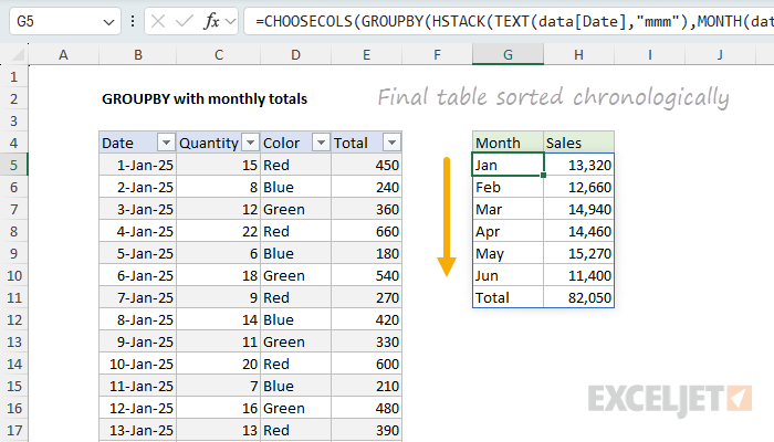
We now have data grouped by month with the month names in chronological order.
Summary of steps
Here's a quick recap of the steps we took:
- Started with a basic GROUPBY using
TEXT(data[Date],"mmm")to create month names from the dates. Works fine, but the sort order is alphabetical (Apr, Feb, Jan...) instead of chronological. - Tried reversing the sort with
sort_order = -1but that just flipped the alphabetical order backwards, which still wasn't what we wanted. - Added month numbers using the HSTACK function because we needed actual numbers (1-12) to sort chronologically.
- Set
sort_order = 2to sort by the month numbers, but this didn't work because GROUPBY was still prioritizing the month names due to its default hierarchical behavior. - Fixed the sorting issue by adding
field_relationship = 1to break the hierarchy and let the month numbers control the sort order. - Used the CHOOSECOLS function to remove the month numbers from the final result since we only need them for sorting, not for display.
Alternative formula #1
As mentioned above, another way to manage the hierarchy is to reorder the row fields so that the month numbers are the first column:
=CHOOSECOLS(GROUPBY(HSTACK(MONTH(data2[Date]),TEXT(data2[Date],"mmm")),data2[Total],SUM),{2,3})
This formula is a bit simpler because we don't need to use the field relationship at all. However, one consequence of moving the month numbers to the first column and then using CHOOSECOLS to remove the first column is that the word "Total" is also removed:
Alternative formula #2
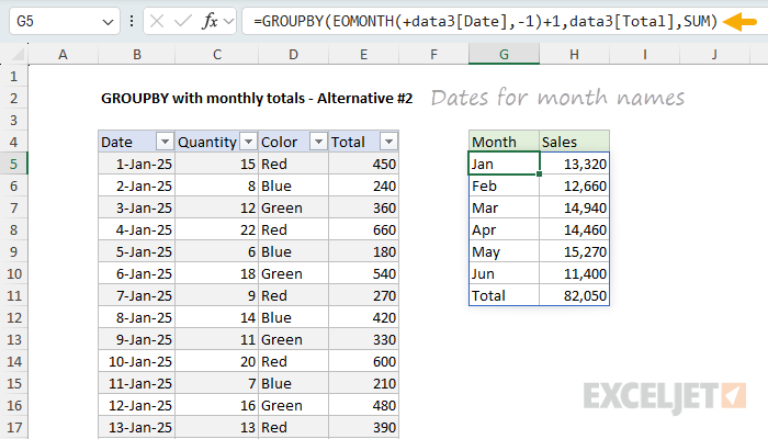
After I published this article, I got an email from a reader with what I think is an even better idea. It is certainly simpler. The basic idea is to leave all of the dates as dates, but to remap them to the first day of each month. The GROUPBY function still groups the data by month as before. The big advantage is that there is no need to sort manually. Because the dates that represent month names are valid dates, they sort naturally in chronological order. You can see this approach in the worksheet below, where the formula in G5 looks like this:
=GROUPBY(EOMONTH(+data3[Date],-1)+1,data3[Total],SUM)
Inside the GROUPBY function, the EOMONTH function is used to get the first day of the month. The effect is to remap all dates to the first of the month so that GROUPBY can group by month as before. As you can see, this formula is much simpler, but there is one extra step: we need to format the month names with the custom date format "mmm".
Because of its simplicity, I think this is the best solution to this problem. However, I think the learning process that the rest of the article goes through is valuable, especially because it shows an example of when the field relationship argument is important.
What is that
+doing in the EOMONTH formula? Some Excel functions, like EOMONTH, resist spilling when provided a range — they won't automatically spill results without extra help. Adding an operator like+in front of the range reference forces Excel to evaluate the expression first, which turns the range into an array of values, which EOMONTH can then process. For more details and a list of functions that have this problem, see: Why some functions won't spill.
Formula for older versions of Excel
The GROUPBY formula only works in the latest version of Excel, which contains dynamic array functions like GROUPBY, HSTACK, and CHOOSECOLS. If you are using an older version of Excel, you will need to use a different approach. I think the easiest approach overall is to enter the month names in column G manually. Then you can use a formula based on SUMPRODUCT in column H to get a monthly total like this:
=SUMPRODUCT(--(TEXT(data2[Date],"mmm")=G5),data2[Total])
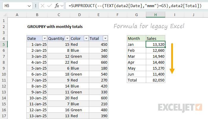
In this worksheet, data2 is the source data in an Excel Table, and G5 is the abbreviated month name. As the formula is copied down, it will return the total for each month. You will then need to calculate a grand total with the SUM function:
=SUM(H5:H10)
This is a fairly simple approach, but it does require manually entering the month names in column G, and the month names will not dynamically update if the source data changes. For more details on how this formula works, see the SUMPRODUCT function page.
Final thoughts
I've been looking for an example where the field relationship argument in the GROUPBY function is needed, and this is a good one. Even after we add the month numbers for sorting, we still can't sort the months chronologically because of the hierarchy that GROUPBY imposes on row fields. We need to set the field relationship argument to 1 to break the hierarchy and let the month numbers control the sort order. It's worth noting also that the core GROUPBY formula is quite simple. It's the process of sorting the months in the correct order that adds complexity.