Summary
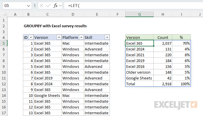
One way to analyze survey results is to use the GROUPBY function. In the example shown, we are creating a table to analyze responses to the question "What version of Excel do you use most?" The core formula in this example is:
=GROUPBY(data[Version],data[Version],COUNTA,0)
This version of the formula shows how GROUPBY can summarize survey responses by Excel version, returning a count for each group. From here, we’ll build on this structure to add percentages, custom sorting, and formatting.
Note: This is a great example of how the GROUPBY function can quickly reveal useful information. At the same time, it also demonstrates how things can get tricky when you want to calculate percentages or customize the sort order. I walk through this process in detail below. By the time we're done, we've implemented a fix for a PERCENTOF error, expanded the formula to use the LET function, added XMATCH, and the SORTBY function for sorting.
Explanation
In May 2025, I ran a survey asking Exceljet newsletter subscribers what version of Excel they use most. This is an important question for Excel learning because the new dynamic array engine has completely changed how many formulas are written. These changes started rolling out after Excel 2019, so users with Excel 2021 or later have access to dynamic array formulas and functions, while those using Excel 2019 and older don't.
The survey generated almost 3,000 responses, making it a perfect dataset to demonstrate Excel's new capabilities. In this article, I'll walk you through using the GROUPBY function to analyze these survey results step by step, showing you how this cool new function can quickly transform raw survey data into useful information.
If you don't have the new GROUPBY function, a regular Pivot Table would also be an excellent way to analyze these results. In many ways, a Pivot Table is easier, but the trade-off is that a Pivot Table needs to be manually refreshed if data changes, whereas the GROUPBY function will automatically update.
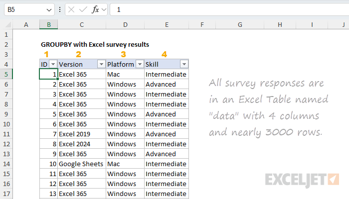
The survey data
The survey data is in an Excel Table called "data" which contains just four columns:
- ID – unique numeric ID for each survey response
- Version – the Excel version most used by the user
- Platform – the platform (Mac or Windows) used
- Skill – the self-reported skill level of the user
Core GROUPBY formula
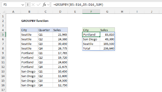
In this example, the goal is to create a table that displays a summary count for each Excel version and the percentage for each count with respect to the total. This is a good job for the GROUPBY function, which is designed to summarize data by grouping rows and aggregating values. As seen in the worksheet below, the core GROUPBY formula looks like this:
=GROUPBY(data[Version],data[Version],COUNTA,0)
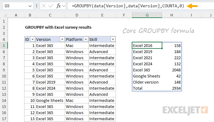
For both row_fields and values, we use the Version column. For the function argument, we use COUNTA, since we are counting text values. This gives us a good start. We don't have a percentage in there yet (or sorting), but we have the correct counts for all versions in the survey data.
Detour
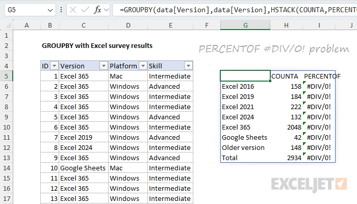
When I set up this formula the first time, my next step was to add the PERCENTOF function to generate a percentage for each count. I also added the HSTACK function so that we have the count and percentage side by side:
=GROUPBY(data[Version],data[Version],HSTACK(COUNTA,PERCENTOF),0)
However, as you can see below, this didn’t work. The COUNT column remained intact, but the PERCENTOF column returned divide-by-zero errors (#DIV/0!).
This led to hacky workarounds on my part and then a quick email to the Excel MVP distribution list, where fellow MVP Mark Proctor was kind enough to set me straight. As Mark pointed out, the PERCENTOF function performs a calculation like this:
=SUM(subset)/SUM(totalset)
But it is the GROUPBY function that provides the values for subset and totalset, and this behavior is fixed. Since I was using the actual version data (as text) for values inside the GROUPBY function, I was literally trying to divide a group of text values by another group of text values like this:
=SUM("value","value","value",...)/SUM("value","value","value","value",...)
As you can imagine, this won’t work. We need to adjust our formula to use numeric values so that PERCENTOF can generate meaningful percentages.
I'm leaving this detour in here to emphasize that even people with a lot of Excel experience get into the weeds often and have to backtrack and take a different route. It's just part of using Excel. 🙃
Back on track with numeric values
To get the PERCENTOF function to work in a case like this, we need to adjust the formula to work with numeric values so that we can calculate a percentage. We don’t need anything fancy. We literally just need a 1 in each row so that we have something to run calculations on. In other words, we want a column of 1s that we can use for values. A column like this isn't available in the source data, so we'll need to create it in the formula.
There are a variety of ways to do this in Excel. One approach is to use a function like SEQUENCE or EXPAND to build an array of 1s. Another approach is to use some kind of Boolean operation on an existing array of values. Below are some code snippets that will create a one-column array filled with 1s with the same number of rows as the survey data:
SEQUENCE(ROWS(data),,1,0)
--(data[Version]=data[Version])
--ISNUMBER(data[ID])
data[ID]^0
In general, I like Boolean operations on source data because they are simple and guarantee we'll end up with an array of the correct size. Since we already have a numeric value in the ID column, I decided to use the last option, data[ID]^0 , since it's clever and elegant, and I'm a sucker for that sort of thing. The idea is to raise the numeric IDs to the power of zero, since any number raised to the power of zero equals one. This works nicely in this problem because the numeric ID is part of the source data. Here is the revised formula:
=GROUPBY(data[Version],data[ID]^0,HSTACK(COUNT,PERCENTOF),0)
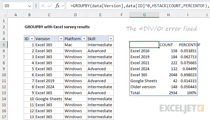
Note that the revised formula provides data[ID]^0 as the values argument. I've also switched from COUNTA to COUNT, since we now have numbers to work with. The SUM function would work just as well, since every number is a 1. Whether you use COUNT or SUM is a personal preference. I like COUNT because it intuitively aligns with "counting results" in this example.
You may not have seen the trick of raising numbers to the power of zero to generate an array of ones. I first ran into several years ago while researching formulas created with the obscure but powerful MMULT function. You can try the formula
=data[ID]^0directly on the worksheet to see how it works.
Dropping the function headers
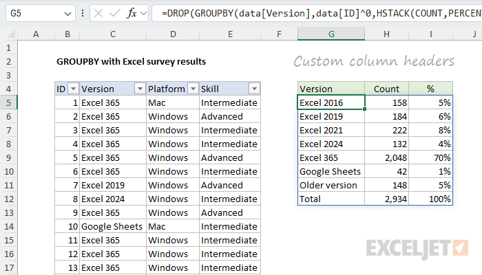
One consequence of adding more than one function with HSTACK is that we get headers above each function, as seen above. The headers appear automatically when you perform more than one calculation with GROUPBY. The headers are useful information in that they quickly tell you what functions are being used, but I like to use my own headers, so I often remove them. We can easily remove the top header row with the DROP function like this:
=DROP(GROUPBY(data[Version],data[ID]^0,HSTACK(COUNT,PERCENTOF),0),1)
In the worksheet below, I'm using the formula above and have added my own column headers in the row above. After we apply some borders and apply percentage number formatting, the table is almost presentable. However, I really want the Excel versions listed in a specific order, and that means we still have work to do.
It's worth noting here that you're on your own when it comes to formatting the output from the GROUPBY function. There are tricks you can use with conditional formatting to auto-format the table, but I'm not using them in this example.
Sorting goal
The main problem at this point is that the version labels are not sorted in any order that makes sense. They are simply sorted alphabetically. I want them to appear in this order:
- Excel 365
- Excel 2024
- Excel 2021
- Excel 2019
- Excel 2016
- Older version
- Google Sheets
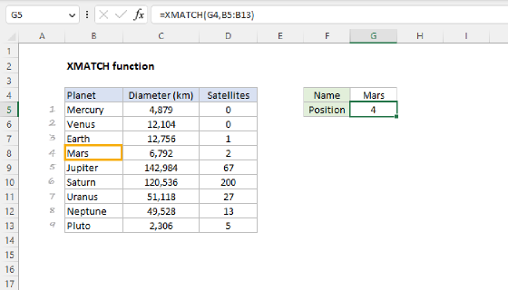
The GROUPBY function has basic controls for sorting columns and ascending or descending orders, but it doesn't provide the custom sorting functionality of the SORTBY function. Instead, we’ll need to build the table with GROUPBY, then feed the result into SORTBY. For the actual sorting, we'll generate an array of sorting values with XMATCH using the order of the list above.
Custom sorting approach
The key feature of Excel’s SORTBY function is that it can sort a range or array using values in another range or array. In other words, if we had an array of numbers that represented the desired sort order, we could use it with SORTBY. Since we already have the Excel versions listed in the desired order on the worksheet in L5:L11, we can generate a custom sorting array with the XMATCH function. The basic idea is to match each version in the GROUPBY table against the sorted list in L5:L11 with the XMATCH function. XMATCH will generate a numeric value for each match, and we’ll use that value for sorting. You can see how this works in the worksheet below, where I've configured XMATCH to demonstrate the concept:
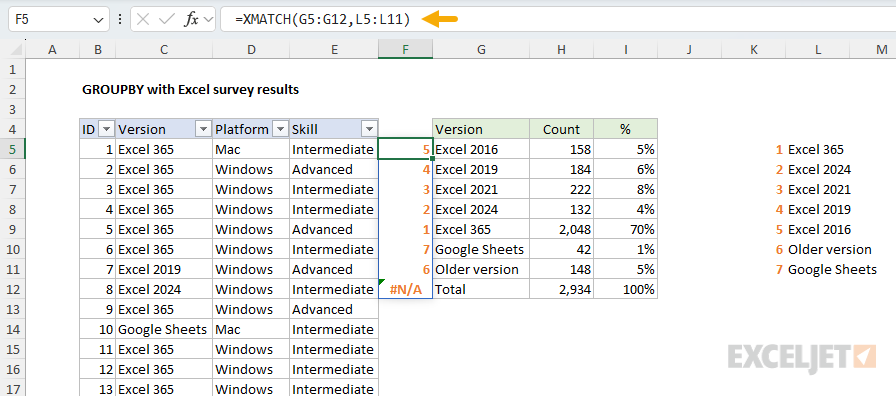
Note that "Total" generates an N/A error because it doesn't appear in our version list. This works fine in this case because the #N/A error automatically sorts to the bottom of the list. The formula above is for illustration only. Below, we move it into the final formula.
Final formula with LET
Since we are sorting the table created by GROUPBY after we have dropped the first row, it will be much easier if we use the LET function to keep our formula organized. Here's the plan: First, we'll build the basic table and drop the header row, as we did above. Next, we'll create a custom sort array with XMATCH. Then we'll feed the table and the custom sort array into the SORTBY function to get a final result. Below is the final formula after implementing LET. Note that we need to use the CHOOSECOLS function to extract just column 1 of the table before we use XMATCH to generate a sorting array:
=LET(
  table,DROP(GROUPBY(data[Version],data[ID]^0,HSTACK(COUNT,PERCENTOF),0),1),
  sort,XMATCH(CHOOSECOLS(table,1), L5:L11),
  result,SORTBY(table, sort),
  result
)
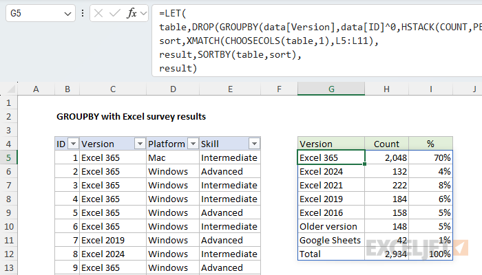
Here is how this formula works:
- In the first step, we build the core table with the GROUPBY function and drop the header row. Then we assign the result to the "table" variable.
- In the next step, we build a sorting array using the XMATCH function and the list of pre-sorted values in L5:L11. The result is an array of numbers we can use to sort by Excel version in a custom order. We assign this array to the variable "sort".
- Next, we feed the table created in step one and the sort array created in step two into the SORTBY function, and assign the sorted table to "result".
- In the last step, we return the sorted table.
Conclusion
The GROUPBY function offers a powerful and flexible way to summarize survey data dynamically in Excel. It works very well with survey data in the format shown, quickly building the equivalent of a lightweight pivot table. With a few modern functions like HSTACK, PERCENTOF, XMATCH, and SORTBY, we can build a fully automated report that updates instantly when new responses are added. Along the way, we saw how small details, like generating numeric inputs for certain calculations, are an important part of getting this formula to work correctly.