LAMBDA append range

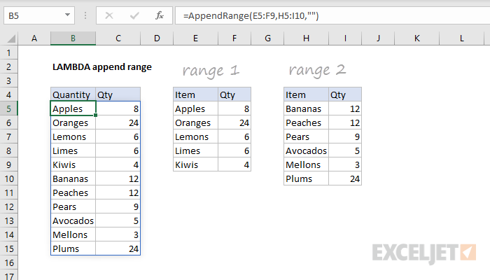
Excel does not provide a function to append ranges, but you can use the LAMBDA function to create a custom function to combine ranges. In the example below, the formula in cell C5 is:

=AppendRange(E5:F9,H5:I10,"null")

This formula combines the two ranges provided (E5:F9 and H5:I10), by appending the second range to the first range, and returns an array of values that spill into B5:C15. The third argument provides a default value to use when the formula runs into errors combining ranges, for example when ranges have different column counts.

Note: this example was created before the VSTACK function and HSTACK function were introduced to Excel. VSTACK combines ranges vertically and HSTACK combines ranges horizontally. These functions are a much easier way to append ranges, but this example is still useful as a way to understand how to approach more complicated problems with dynamic array formulas.

Explanation

You can use the LAMBDA function to create a custom function to combine ranges. In the example below, the formula in cell C5 is:

=AppendRange(E5:F9,H5:I10,"null")

This is a custom function created with LAMBDA, based on several Excel functions, including INDEX, SEQUENCE, IFERROR, ROWS, COLUMNS, and MAX. Holding the whole thing together are LAMBDA and LET:

=LAMBDA(range1,range2,default,
  LET(
  rows1,ROWS(range1),
  rows2,ROWS(range2),
  cols1,COLUMNS(range1),
  cols2,COLUMNS(range2),
  rowindex,SEQUENCE(rows1+rows2),
  colindex,SEQUENCE(1,MAX(cols1,cols2)),
  result,
  IF(
    rowindex<=rows1,
    INDEX(range1,rowindex,colindex),
    INDEX(range2,rowindex-rows1,colindex)
  ),
  IFERROR(result,default)
  )
)

This formula is based on a simplified formula explained here. It's a good example of how the LAMBDA function and LET function work well together. Inside the LET function, the first six lines of code simply assign values to variables. Once values are assigned, these variables drive the output of the function.

The core logic of the formula, the code that builds the combined array, is here:

  result,
  IF(
    rowindex<=rows1,
    INDEX(range1,rowindex,colindex),
    INDEX(range2,rowindex-rows1,colindex)
  ),
  IFERROR(result,default)
  )

This code can be tricky to read, especially if you're new to LAMBDA functions and dynamic array formulas in general. With line breaks added for readability, it's tempting to read it like a loop, with rowindex as an incrementing counter, but in reality, rowindex is not one value, but an array of 11 values, created with the SEQUENCE function earlier:

rowindex,SEQUENCE(rows1+rows2) // assigns {1;2;3;4;5;6;7;8;9;10;11}

The IF function tests the values in rowindex all at once. If rowindex is less than or equal to the count of the rows in range1 (5), INDEX fetches rows from range1. If the rowindex is greater than 5, INDEX fetches rows from range2. If we expand the values of the variables, the code looks something like this:

=IF({1;2;3;4;5;6;7;8;9;10;11}<=5,
INDEX(E5:F9,{1;2;3;4;5;6;7;8;9;10;11},{1,2}),
INDEX(H5:I10,{1;2;3;4;5;6;7;8;9;10;11}-5,{1,2}))

This code can be tested directly on a worksheet, and it will return the same result as the formula.

The array that IF and INDEX create is assigned to the variable result, which is returned as a final value by the formula through the IFERROR function. This is done as a way to catch errors that occur when ranges of different column counts are combined. For example if you combine a two-column range with a one-column range, INDEX will throw an error when it tries to get values from column 2, since column 2 does not exist. In this case, the default value will be output instead of an error.