LAMBDA Function

The LAMBDA function provides a way to create a custom function in Excel. Once defined and named, a LAMBDA function can be used anywhere in a workbook, just like a built-in function. LAMBDA functions can be very simple or quite complex, combining many Excel functions into one formula. A custom LAMBDA function does not require VBA or macros.

The key idea behind LAMBDA is to separate a calculation from the cells it works on. An ordinary formula like =B5*C5 is tied to specific cells. With LAMBDA, you replace the cell references with names called parameters, then write the calculation with those names:

=LAMBDA(x,y,x*y)

Here, x and y are parameters, and x*y is the calculation. The parameters are placeholders for values that will arrive later. This means a LAMBDA is a calculation that is ready to run but has no values to work with yet. Something needs to supply the values, and this happens in one of three ways:

1. You supply the values yourself in a second set of parentheses. This is how a LAMBDA is called directly on the worksheet.
2. You give the LAMBDA a name in the Name Manager, then call it by name like any other function. This is how a LAMBDA becomes a custom function.
3. You hand the LAMBDA to another function like MAP or BYROW, which supplies the values for you.

Everything on this page is a variation on one of these three ideas.

LAMBDA is available in Excel 2024+ and Excel 365.

Key features

• Creates a custom, reusable function without VBA or macros
• Parameters come first, and the calculation is always the last argument
• Can be tested on the worksheet by supplying values in a second set of parentheses
• Named in the Name Manager, then called like any built-in function
• The logic lives in one place, so one update in the Name Manager updates every formula that uses the function
• Can be passed to functions like MAP, BYROW, SCAN, and REDUCE
• Supports optional arguments (with ISOMITTED) and recursion

Table of contents

• Basic examples
• Create a custom function step by step
• Volume of a sphere
• Count words
• LAMBDA with LET
• LAMBDA inside other functions
• Optional arguments
• Recursive LAMBDA
• Number to words
• LAMBDA naming rules
• Notes

Basic examples

The simple LAMBDA below has one parameter, x, and a calculation that squares x. Entered in a cell like this, it returns a #CALC! error:

=LAMBDA(x,x^2) // returns #CALC!

The error does not mean the formula is broken. It means the LAMBDA has not been given a value for x, so there is nothing to calculate. To supply a value directly, add a second set of parentheses at the end:

=LAMBDA(x,x^2)(5) // returns 25
=LAMBDA(x,x^2)(A1) // squares the value in A1

When a LAMBDA has more than one parameter, values are matched to parameters by position. In the formula below, 3 goes to x and 4 goes to y:

=LAMBDA(x,y,x*y)(3,4) // returns 12

Once a LAMBDA has been given a name in the Name Manager, it can be called by that name. For example, after the first LAMBDA above is named "Square":

=Square(5) // returns 25
=Square(A1) // squares the value in A1

Finally, a LAMBDA can be handed to another function. Below, the MAP function runs the same LAMBDA once for each value in an array, supplying the value for x each time:

=MAP({1,2,3},LAMBDA(x,x^2)) // returns {1,4,9}

Notice the LAMBDA is identical in all three cases. The only thing that changes is where the value for x comes from.

Create a custom function step by step

In computer programming, the term "lambda" refers to an anonymous function, which is a function defined without a name. This is a good description of how LAMBDA is used in Excel. LAMBDA functions are typically created and debugged in the formula bar on a worksheet, as a generic (unnamed) formula. Once the generic version has been tested, it is moved into the Name Manager, where it is given a name that can be used anywhere in the workbook.

There are four basic steps to create and use a custom LAMBDA function:

1. Verify the logic you will use with a standard formula
2. Create and test a generic (unnamed) LAMBDA version of the formula
3. Name and define the LAMBDA formula with the Name Manager
4. Call the new custom function with the defined name

To illustrate how this works, let's begin with a very simple formula that multiplies x by y:

=x*y // multiply x and y

Of course, we don't need a custom function to multiply two numbers in Excel. The * operator and the PRODUCT function work fine. The point here is to show how LAMBDA works with the simplest possible calculation. The examples below include scenarios where a reusable LAMBDA has more value.

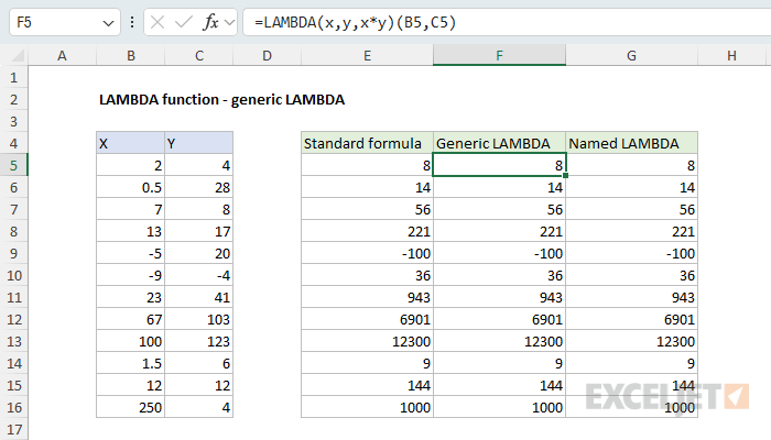
In Excel, this formula would typically use cell references. In the worksheet shown above, the formula in E5, copied down, is:

=B5*C5 // with cell references

This is step 1. The formula works fine, so we are ready to move on to step 2, a generic LAMBDA version of the formula. The first thing to consider is if the formula requires inputs (parameters). In this case, the answer is "yes": the formula requires a value for x, and a value for y. This means we need to start off the LAMBDA with parameters for each input:

=LAMBDA(x,y  // begin with input parameters

Next, we need to add the actual calculation, x*y:

=LAMBDA(x,y,x*y)

At this point, the formula is complete, but if you enter the formula like this, you'll get a #CALC! error. This happens because the formula has no input values to work with since there are no longer any cell references. To test the formula, we need to use a special syntax like this:

=LAMBDA(x,y,x*y)(B5,C5) // testing syntax

This syntax, where values are supplied at the end of a LAMBDA function in a separate set of parentheses, is unique to LAMBDA functions. It allows the formula to be tested and used directly on the worksheet without a custom name. In the screen below, you can see that the generic LAMBDA function in F5 returns exactly the same result as the original formula in E5:

Excel is picky about this syntax. The second pair of parentheses must follow the first pair with no space. If you add a space, you'll get a #VALUE! error, or Excel will refuse to accept the formula.

We are now ready for step 3, which is to name the LAMBDA function with the Name Manager. First, copy the formula, but do not include the testing values at the end. Next, open the Name Manager (Formulas > Name Manager, or the keyboard shortcut Control + F3), and click New.

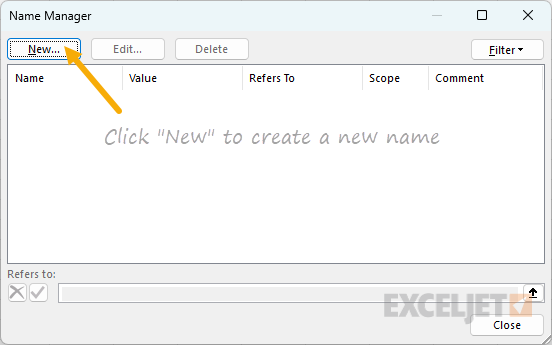
In the New Name dialog, enter the name "Multiply", leave the scope set to "Workbook", and paste the formula you copied into the "Refers to" input area. (Tip: Use the tab key to navigate to the "Refers to" field).

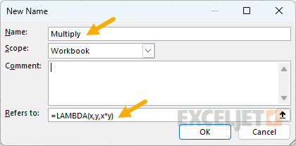
Make sure the formula begins with an equals sign (=), then press the "OK" button to save and close the Name Manager. Now that the LAMBDA formula has a name, we can move on to step 4 and use the new function in the workbook like any other function. In the screen below, the formula in G5, copied down, is:

=Multiply(B5,C5)

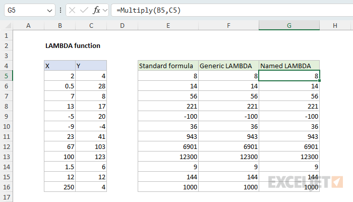
The new custom function returns the same result as the other two formulas. Notice that the standard formula in column E, the generic LAMBDA in column F, and the named LAMBDA in column G are the same calculation in three different forms.

It is extremely difficult to edit a formula in the input area of the Name Manager. I don't recommend it if you want to preserve your sanity. Instead, always edit and test the formula on the worksheet first, then copy and paste the formula into the Name Manager. Also, LAMBDA names have certain restrictions you should be aware of.

Volume of a sphere

In this example, we'll run through the same four steps more quickly to convert a more practical formula into a custom function. The general Excel formula for calculating the volume of a sphere is:

=4/3*PI()*A1^3 // volume of sphere

where A1 represents the radius. Notice this formula only requires one input (radius) to calculate volume, so our LAMBDA function will only need one parameter (r), which will appear as the first argument. Here is the formula converted to a generic LAMBDA, with B5 supplied as the radius for testing:

=LAMBDA(r,4/3*PI()*r^3)(B5) // generic lambda

Once we confirm that the generic LAMBDA returns the same results as the standard formula, the next step is to name the LAMBDA with the Name Manager, as explained above. The name used for a LAMBDA function can be any valid Excel name. In this case, we'll name the formula "SphereVolume" and paste in the LAMBDA without the testing syntax:

=LAMBDA(r,4/3*PI()*r^3)

In the worksheet below, column D contains the standard formula, column E contains the generic LAMBDA, and column F contains the new custom function. The formula in F5, copied down, is:

=SphereVolume(B5)

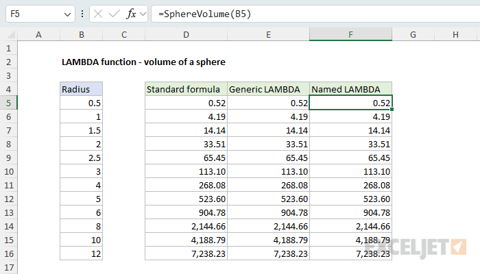
The results from the custom SphereVolume function are exactly the same as the results from the other two formulas. The difference is that a formula with SphereVolume is easy to read and easy to write, and nobody needs to remember the math.

Count words

One of the key benefits of a custom LAMBDA function is that the logic contained in the formula exists in just one place. This means there is just one copy of code to update when fixing problems or updating functionality, and changes will automatically propagate to all instances of the LAMBDA function in a workbook. This example shows how that works.

Excel doesn't have a function to count words, but you can count words in a cell with a formula based on the LEN and SUBSTITUTE functions like this:

=LEN(TRIM(A1))-LEN(SUBSTITUTE(A1," ",""))+1

Read the detailed explanation here. This formula only requires one input: the text that contains words. In our LAMBDA function, we'll name this argument text. Here is the formula converted to LAMBDA:

=LAMBDA(text,LEN(TRIM(text))-LEN(SUBSTITUTE(text," ",""))+1)

Notice text appears as the first argument, and the calculation is the second and final argument. After we test the formula and name it "CountWords" in the Name Manager, we can count the words in cell B5 like this:

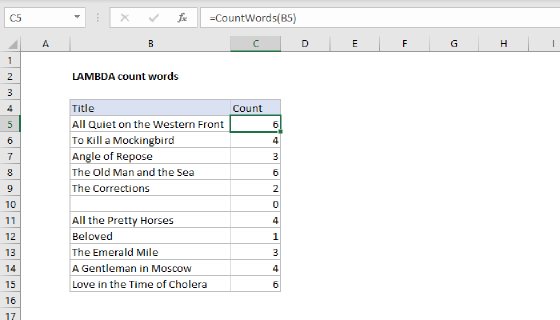
=CountWords(B5)

This is much simpler than the original formula above. However, there is a problem. The formula returns an incorrect count of 1 when a cell is empty. This is a bug caused by always adding 1 in the formula, even when there is no text. We can fix this problem by replacing +1 with a Boolean expression that returns 1 only when the cell contains text. To update CountWords, we again need to use the Name Manager:

1. Open the Name Manager
2. Select the name "CountWords" and click "Edit"
3. Replace the "Refers to" code with this formula:

=LAMBDA(text,LEN(TRIM(text))-LEN(SUBSTITUTE(text," ",""))+(LEN(TRIM(text))>0))

Once the Name Manager is closed, CountWords works correctly on empty cells. In the worksheet below, the formula in D5, copied down, is still =CountWords(B5), but the count for the empty cell in B10 is now zero:

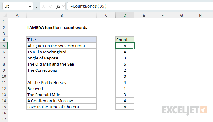
Updating the code once in the Name Manager updates all instances of the CountWords formula at once. This is a key benefit of custom functions created with LAMBDA: formula updates can be managed in one place.

For a full walkthrough of this example, see LAMBDA count words.

LAMBDA with LET

The LET function is often used together with the LAMBDA function. LET provides a way to declare variables and assign values in a formula. This makes more complicated formulas easier to read by reducing redundant code. The two functions fit together naturally: LAMBDA names the inputs to a formula, and LET names the steps inside it.

A LET formula is also a good starting point for a custom function. For example, the formula below converts inches to feet and inches, so that 70 becomes 5' 10":

=LET(
  input,B5,
  n,ROUND(ABS(input),0),
  sign,IF(input<0,"-",""),
  feet,INT(n/12),
  inches,MOD(n,12),
  sign&feet&"' "&inches&""""
)

Notice that the cell reference B5 appears just once, on the first line, where it is assigned to the variable input. Every other line works with input. This makes the conversion to LAMBDA simple: remove the first line of LET, and make input a LAMBDA parameter:

=LAMBDA(input,
  LET(
    n,ROUND(ABS(input),0),
    sign,IF(input<0,"-",""),
    feet,INT(n/12),
    inches,MOD(n,12),
    sign&feet&"' "&inches&""""
  )
)

The rest of the formula does not change. After we name this LAMBDA "InchesToFeet" in the Name Manager, the formula in D5 of the worksheet below, copied down, is:

=InchesToFeet(B5)

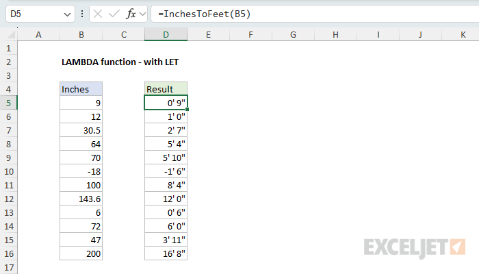
The eight-line formula is now a one-word function. Anyone can use InchesToFeet without understanding how the conversion works, and if the logic needs to change, there is one place to change it.

The same approach works for more complex formulas. If a formula you want to reuse is long and nested, or refers to the same cell more than once, restructure it with LET first: assign each input cell to a variable at the top, then name the key steps that follow. Once every cell reference lives on its own line at the top of LET, the conversion to LAMBDA is the same as above: remove those lines, and make each input a LAMBDA parameter. For a step-by-step guide to restructuring a formula with LET, see Converting a formula to LET.

LAMBDA inside other functions

So far, each LAMBDA on this page has been given a name. However, many people encounter LAMBDA for the first time in a different setting: inside another function. Excel has a group of functions designed to work with LAMBDA: MAP, BYROW, BYCOL, SCAN, REDUCE, and MAKEARRAY. Each of these functions takes a LAMBDA as its last argument. The function loops over an array and calls the LAMBDA once for each value (or each row, or each column), and supplies the values for the parameters as it goes. A LAMBDA used this way is never named. It exists only inside the formula.

In the worksheet below, the goal is to return "Pass" when both test scores are at least 70, and "Fail" if not. With a formula copied down the column, this is a job for the IF function and the AND function:

=IF(AND(C5>=70,D5>=70),"Pass","Fail")

But what if we want a single dynamic array formula that returns all 12 results at once? The obvious approach is to give the formula above the full ranges, C5:C16 and D5:D16. But this won't work, because AND aggregates all values into a single result, and the formula returns a single "Fail". The MAP function solves this problem. The formula in F5 is:

=MAP(C5:C16,D5:D16,LAMBDA(a,b,IF(AND(a>=70,b>=70),"Pass","Fail")))

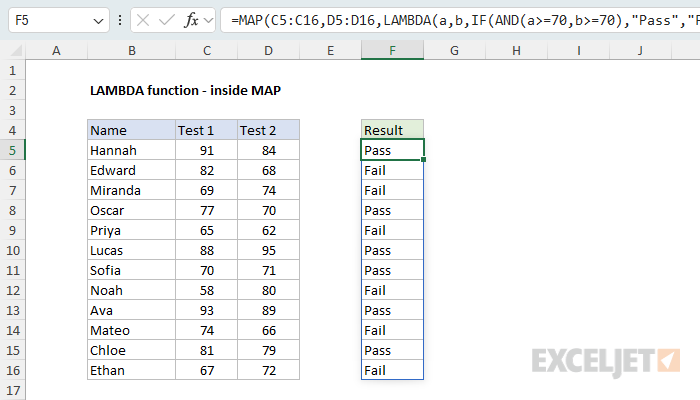
Look closely at the LAMBDA. The calculation is the original formula, with a and b in place of C5 and D5. MAP takes one value at a time from C5:C16 and D5:D16, passes the two values into the LAMBDA as a and b, and collects the results. Because AND only sees one pair of values at a time, it works as intended, and the 12 results spill into the range F5:F16.

The BYROW function works the same way, except the LAMBDA receives an entire row. In the worksheet below, the goal is to calculate the spread between the highest and lowest quiz score for each person. The formula in H5 is:

=BYROW(C5:F16,LAMBDA(row,MAX(row)-MIN(row)))

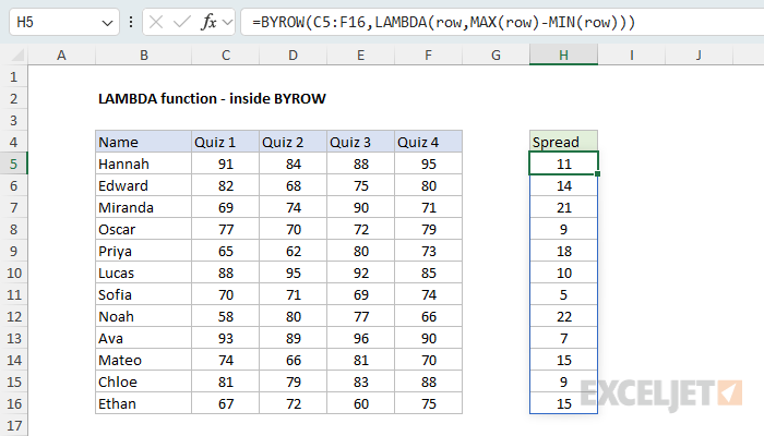
BYROW calls the LAMBDA 12 times, once for each row in C5:F16. Each time, row holds the four scores in one row, and the calculation returns the maximum value minus the minimum value.

When the calculation is nothing more than a single function, Excel allows a shortcut: you can supply the function name alone in place of a LAMBDA. This is sometimes called an "eta lambda". Both formulas below return the same result:

=BYROW(C5:F16,LAMBDA(row,SUM(row))) // sum each row
=BYROW(C5:F16,SUM) // same result

A custom function created with LAMBDA works the same way. For example, =MAP(B5:B15,CountWords) runs the CountWords function above on each cell in B5:B15. For more details and examples, see the pages for MAP, BYROW, BYCOL, SCAN, REDUCE, and MAKEARRAY.

Optional arguments

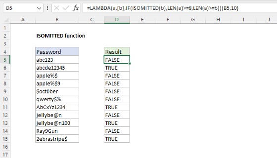
By default, all arguments in a LAMBDA function are required. To make an argument optional, enclose the parameter name in square brackets, then use the ISOMITTED function inside the calculation to check if a value was provided. ISOMITTED returns TRUE when an argument has not been supplied.

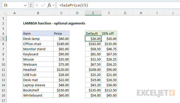
In the worksheet below, the custom function "SalePrice" applies a discount to a price. The discount argument is optional, and defaults to 10%. The LAMBDA used to define SalePrice looks like this:

=LAMBDA(price,[discount],
  IF(ISOMITTED(discount),price*0.9,price*(1-discount))
)

When discount is omitted, ISOMITTED returns TRUE, and the function returns 90% of price. When discount is provided, the function uses the value provided. The formulas in E5 and F5 are:

=SalePrice(C5) // default 10% discount
=SalePrice(C5,0.25) // 25% discount

Optional arguments must come after required arguments. For more details, see the ISOMITTED function.

Recursive LAMBDA

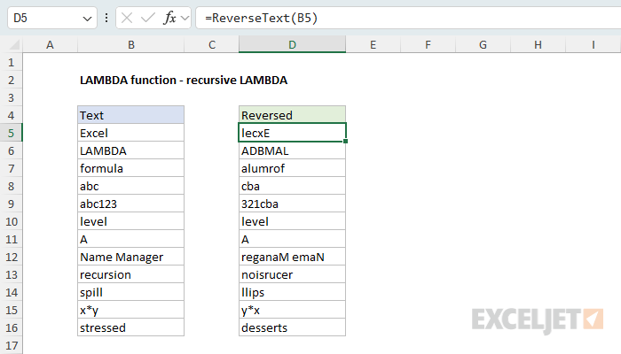
A custom LAMBDA function can call itself by name. This is called recursion, and it provides a way to repeat a calculation an unknown number of times. A recursive function has two parts: a test that decides when to stop, and a call to itself with a smaller version of the problem. For example, the custom function "ReverseText" reverses a text string:

=LAMBDA(text,
  IF(LEN(text)<=1,text,
    RIGHT(text)&ReverseText(LEFT(text,LEN(text)-1))
  )
)

The IF function controls the process. When text contains one character or less, there is nothing to reverse, and the function returns text as-is. Otherwise, the function takes the last character with the RIGHT function, and joins it to the result of calling ReverseText on the rest of the text. With the text "abc", the calls unfold like this:

=ReverseText("abc")
="c"&ReverseText("ab")
="c"&"b"&ReverseText("a")
="c"&"b"&"a"
="cba"

In the worksheet below, the formula in D5, copied down, is:

=ReverseText(B5)

Recursive formulas are powerful, but they can be very confusing if you don't have a background in programming, partly because Excel gives you no tools to step through the formula and watch the recursion happen. In many cases, there is another way to solve the problem without recursion, using dynamic array formulas.

There are a few other things to keep in mind with recursive LAMBDA functions:

• A recursive LAMBDA can't be tested on the worksheet with the testing syntax, because a LAMBDA without a name has no way to call itself. It must be defined in the Name Manager first.
• Use the IF function for the test that ends the recursion. The IFS function and the SWITCH function evaluate all of their arguments, including the recursive call, so the function never stops calling itself and returns a #NUM! error.
• The REDUCE function often replaces recursion. It loops over a list of values and accumulates a result, with no function calling itself.

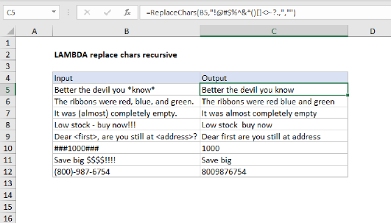
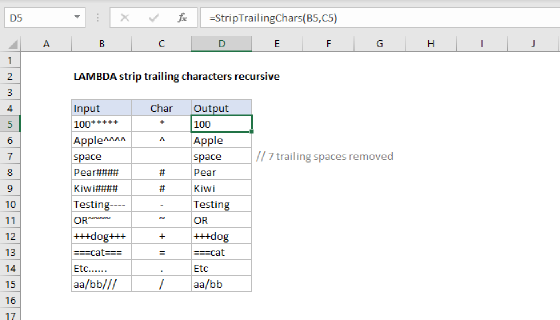
For more examples of recursion, see LAMBDA replace characters recursive and LAMBDA strip trailing characters recursive.

Number to words

Custom LAMBDA functions can be quite sophisticated, and they can even include sub-routines that encapsulate reusable logic. In the worksheet below, "NumberToWords" is a custom lambda that will convert a number like 123 into "One hundred twenty three" or "One hundred twenty three dollars" when currency is specified as USD:

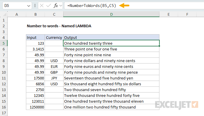
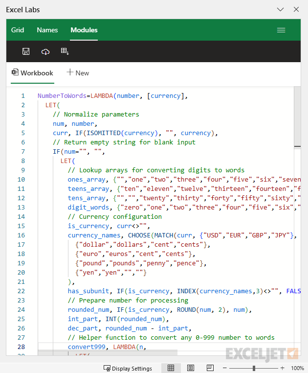
This is a complex problem in Excel, usually handled with VBA (Visual Basic). In this case, however, all required logic is contained in a single LAMBDA with about 80 lines of code. This is what the code looks like in the Excel Labs Advanced Formula Environment:

You can find the full source code and a downloadable workbook on this page.

LAMBDA naming rules

When naming a custom LAMBDA function in Excel, there are some restrictions you should be aware of:

1. The name must be between 1 to 255 characters long.
2. The name must start with a letter (A-Z, a-z) or an underscore (_).
3. The name must not contain spaces or special characters like @, !, #, $, %, etc.
4. The name must not be a cell reference like A1, C2, X100, etc.
5. The name must not conflict with an existing Excel function like SUM, COUNT, TEXT, etc.

The last point, 5, is especially important. While Excel will stop you from breaking the first 4 rules, it will not prevent you from naming your custom LAMBDA after an existing function. If you break this rule, the name will be created, but your custom function will never be invoked since Excel will default to existing function names. The result can be very confusing. Avoid this trouble by making sure your custom function name is unique.

Custom LAMBDA names are not case-sensitive. The names "MYFUNCTION", "MyFunction", and "myfunction" all refer to the same function, and Excel will change the name you type in a formula to match the capitalization used in the Name Manager.

A related question is how to tell a custom function from a built-in function when you see it in a formula. The convention used on this site is to name custom functions with capitalized words, like CountWords or SphereVolume. Excel always displays built-in functions in uppercase, so a name in mixed case is always a custom function. This also makes the names easier to read, and since Excel corrects the capitalization when you enter a formula, =countwords(B5) becomes =CountWords(B5) as soon as you press Enter, which confirms that the name was found.

Notes

• A LAMBDA entered in a cell without input values returns a #CALC! error. Add values in a second set of parentheses to test, or define a name.
• A custom function called with too many arguments, or too few required arguments, returns a #VALUE! error.
• The calculation must be the last argument in LAMBDA. A LAMBDA can have up to 253 parameters.
• Parameter names follow the same basic rules as names in the LET function: they can't contain spaces or periods, and they can't look like a cell reference (for example, x1 or ab12).
• A custom function belongs to the workbook where it is defined. To use the function in another workbook, copy a formula in a worksheet that uses the function into the other workbook, and Excel will bring the name along.
• A formula that calls a custom function will return a #NAME? error when the function is not defined in the workbook, or when the workbook is opened in a version of Excel without LAMBDA.
• A recursive LAMBDA that calls itself too many times returns a #NUM! error.
• LAMBDA is available in Excel 2024+ and Excel 365.