MAP Function

The MAP function runs a LAMBDA formula on each value in an array and returns the results in an array of the same size and shape. If you give MAP a 3 x 4 range of 12 cells, it will return a 3 x 4 array of 12 results that spill onto the worksheet.

The name MAP comes from the mathematical concept of a "map", which is a function that relates each point in one set to a point in another set, the way a geographical map relates points on paper to places in the real world. MAP works by "mapping" each value in an array to a new value created with LAMBDA.

In the context of Excel formulas, the easiest way to think about MAP is this: write a formula for one cell, and MAP runs it on every cell in a given range. The LAMBDA is the formula, with a variable in place of the cell reference.

Because Excel can already natively apply a function to a range of cells without MAP, one of the trickiest aspects of MAP is knowing when to use it. The examples below cover the three common reasons a formula needs MAP. See When to use MAP for a summary.

Key features

• Runs a LAMBDA once on each value in an array and returns one result per value, in the same shape: a range of 4 rows and 3 columns returns 4 rows and 3 columns.
• Accepts more than one array. The LAMBDA takes one parameter per array, in order, and MAP reads the arrays in step, so they should be the same size.
• The LAMBDA must return a single value for each item. A LAMBDA that returns an array makes MAP return #CALC!.
• Given a range, MAP passes each value as a cell reference, so functions that need a reference, like SUBTOTAL, will work inside the LAMBDA.
• Accepts a function name, like MAX, or a named LAMBDA, in place of a LAMBDA.
• Isn't needed when a formula already spills. Use it when the formula for one cell won't spill on its own.

Table of contents

• Basic examples
• Test each value with AND
• Larger of two values in each row
• When to use MAP
• Check each cell for a list of words
• List the matching words in each cell
• Count or sum values in each cell
• Get initials for a seating chart
• Count visible rows with criteria
• Running count of each value
• Notes

Basic examples

MAP takes one or more arrays, followed by a LAMBDA, which is always the last argument. With one array, the LAMBDA has one parameter, and MAP passes each value to it in turn:

=MAP(range,LAMBDA(x,x*2)) // same as =range*2
=MAP(range,LAMBDA(x,AND(x>=10,x<=20))) // AND on each value
=MAP({1,2;3,4},LAMBDA(x,x*10)) // returns {10,20;30,40}

With two arrays, the LAMBDA has two parameters. MAP reads the arrays in step: the first value from each array goes in together, then the second, and so on. Adding another array means adding another variable in the LAMBDA:

=MAP(range1,range2,LAMBDA(a,b,a+b)) // add two arrays
=MAP({1,2,3},{10,20,30},LAMBDA(a,b,a+b)) // returns {11,22,33}
=MAP(range1,range2,range3,LAMBDA(a,b,c,a+b+c)) // add three arrays

Instead of a LAMBDA, you can give MAP the name of a function, or of a named LAMBDA like CountWords:

=MAP(range1,range2,range3,MAX) // largest of the 3 values
=MAP(range,CountWords) // count words in each cell with named function

Test each value with AND

The most common reason to use MAP is when you want to process a range with a function like AND, OR, MAX, or MIN. The problem is that these functions return a single result, so they interrupt certain range operations that are meant to spill. For example, in the worksheet below, the goal is to test whether each score is between 70 and 89. For one score, the formula is =AND(C5>=70,C5<=89), which works fine. However, if we try to test all the scores at once by using ranges instead, the formula returns just one result:

=AND(C5:C16>=70,C5:C16<=89) // returns single FALSE

This happens because AND always returns one result, as you can see in cell G5. To work around this problem, use a variable in place of C5, wrap the formula in a LAMBDA, and give MAP the range. The formula in E5 is:

=MAP(C5:C16,LAMBDA(x,AND(x>=70,x<=89)))

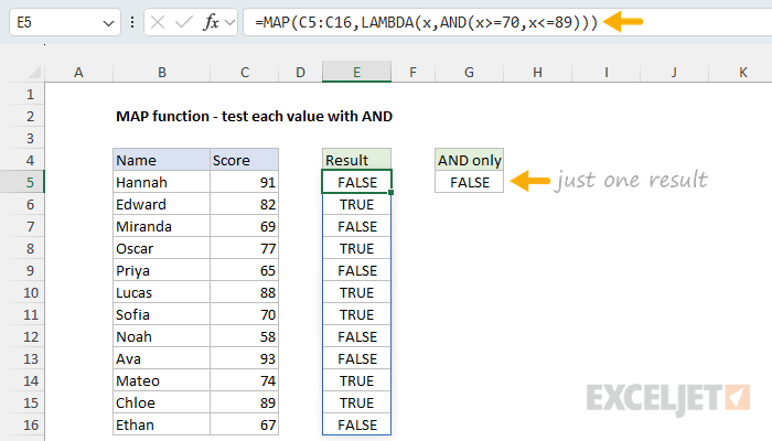
MAP passes each score in C5:C16 to x, one at a time, and AND returns TRUE or FALSE for that score. Because AND only sees one score at a time, it works correctly, and the 12 results spill into E5:E16.

Boolean logic is another way to spill results without MAP: =(C5:C16>=70)*(C5:C16<=89) returns 1 or 0 for each score. MAP lets you keep the AND formula you would write for one cell.

Because the result is one TRUE or FALSE per row, the same MAP formula can work nicely as the include argument of the FILTER function. This formula returns the names with a score between 70 and 89:

=FILTER(B5:B16,MAP(C5:C16,LAMBDA(x,AND(x>=70,x<=89))))

For more on this pattern, see MAP with AND and OR logic.

Larger of two values in each row

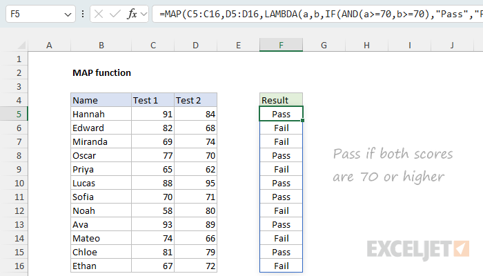
In the worksheet below, students who took a retest keep the higher of their two scores. Because the scores are in two columns, MAP gets two arrays, one for each column. The formula in F5 is:

=MAP(C5:C16,D5:D16,LAMBDA(a,b,MAX(a,b)))

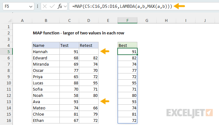
With two arrays, the LAMBDA takes two parameters, in the same order as the arrays: a is the test score and b is the retest score. MAP reads the arrays in step, so the two scores in each row travel together, and MAX returns the larger one. Hannah and Ava didn't take a retest, and MAX ignores the empty cell, so their test score is the result. Like AND, MAX will truncate certain array operations without MAP. The formula =MAX(C5:C16,D5:D16) returns just 95, the single largest score in both columns.

You are free to name the variables inside the LAMBDA anything you like, but you must take care not to use names that could conflict with cell references. For example, a and b work fine, but a1 and b1 will not work. A name that hints at the value makes a formula easier to follow, like t for text and n for name in the examples below.

When the LAMBDA does nothing but pass its parameters to one function, you can give MAP the function name instead (an eta lambda). This formula returns the same result:

=MAP(C5:C16,D5:D16,MAX)

Because the two columns sit side by side, =BYROW(C5:D16,MAX) also works. However, an advantage of the MAP function over BYROW is that you can pick specific columns out of a larger range, even columns that aren't next to each other, and apply a function to them one row at a time.

When to use MAP

Because Excel already runs most formulas on every value in a range (a behavior called lifting), MAP is not necessary for many operations. For example, both of these formulas multiply the values in C5:C16 by two and return the same result:

=C5:C16*2
=MAP(C5:C16,LAMBDA(x,x*2))

When a formula like this spills on its own, you don't need MAP. Use MAP when the formula you would write for one cell won't spill when you give it a range. There are three common reasons why that might happen:

1. The formula uses a function that returns one result for a whole range, like AND, OR, MAX, MIN, or SUM. See the two examples above.
2. The formula already works through a list for each value, like a list of words to look for, or the parts of a name split at each space. When you give the formula a range, Excel tries to pair the range with the list, or returns only part of each result, instead of running the full formula on each cell. See Check each cell for a list of words and the examples after it.
3. The formula needs each value as a cell reference. Functions like SUBTOTAL, and ranges built from the current cell like B5:c, only work with references. Given a range, MAP passes each value as a reference. See Count visible rows with criteria and Running count of each value.

Note that some older functions, like EDATE and EOMONTH, return #VALUE! when you give them a range. You can use MAP to work around this problem like this:

=MAP(B5:B16,LAMBDA(d,EDATE(d,1))) // add one month to each date

However, a plus sign (+) in front of the range is shorter, and it works for the whole group of functions that have this limitation: =EDATE(+B5:B16,1). For details, see Why some Excel functions won't spill.

Check each cell for a list of words

In the worksheet below, the goal is to flag the comments that mention any of the words in F5:F7. For one comment, the formula is =OR(ISNUMBER(SEARCH(F5:F7,B5))). SEARCH looks for all three words and returns three results: a number for each word it finds, and #VALUE! for each word it doesn't. ISNUMBER returns TRUE for each number, and OR returns TRUE if any word was found. The formula in D5 runs it on every comment at the same time:

=MAP(B5:B14,LAMBDA(t,OR(ISNUMBER(SEARCH(F5:F7,t)))))

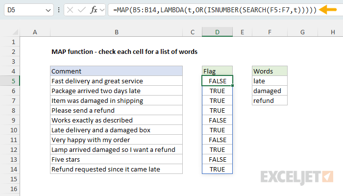
MAP passes each comment in B5:B14 to t (for text), one at a time, and the formula returns TRUE if that comment contains any of the words.

Why not give the formula the whole range, B5:B14? Well, there are two problems. First, OR returns a single result, just like AND in the first example. Second, the formula already uses an array: the three words in F5:F7 become {"late";"damaged";"refund"} when the formula is evaluated. When given a second array, SEARCH pairs the two arrays item by item instead of checking every combination: comment 1 with "late", comment 2 with "damaged", comment 3 with "refund", and #N/A for the rest. Even without OR, =ISNUMBER(SEARCH(F5:F7,B5:B14)) returns FALSE for every comment in this worksheet. In contrast, MAP gives the formula one comment at a time, so each comment is checked against the list of words correctly.

SEARCH isn't case-sensitive, so "Late" matches "late". It also finds words inside other words: "late" matches "chocolate".

For more on this formula, see Cell contains one of many things.

List the matching words in each cell

It's important to remember that MAP needs a single result for each item. If the LAMBDA returns an array of results, MAP returns #CALC!. To illustrate, let's look at the example below.

Building on the formula above, the next step is to list the words each comment contains. The FILTER function can return the matching words, but if we use FILTER by itself in the LAMBDA, MAP returns a single #CALC! error:

=MAP(B5:B14,LAMBDA(t,FILTER(F5:F7,ISNUMBER(SEARCH(F5:F7,t)),""))) // returns #CALC!

This happens because three of the comments contain two of the words, so FILTER returns two results for them. With the same data, we can use a formula like this in cell D5 instead:

=MAP(B5:B14,LAMBDA(t,TEXTJOIN(", ",TRUE,FILTER(F5:F7,ISNUMBER(SEARCH(F5:F7,t)),""))))

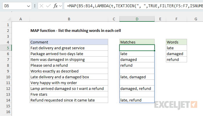
For each comment, FILTER returns the words that SEARCH finds, or an empty string ("") when there are none. Because there might be more than one word found, we need a way to force a single result. The TEXTJOIN function solves the problem by joining the words into one text value, separated by a comma and a space. This is the general fix for #CALC! in MAP: reduce each item's results to one value.

To return only the first word that matches, use XLOOKUP in the LAMBDA instead of FILTER: XLOOKUP(TRUE,ISNUMBER(SEARCH(F5:F7,t)),F5:F7,""). You can use this approach to assign categories based on keywords, as explained in Categorize text with keywords. For more on listing matches, see Get all matches cell contains.

Count or sum values in each cell

Sometimes one cell holds several values, separated by commas. In the worksheet below, each student's quiz scores are in one cell, and the goal is to count and total the scores. The formulas in E5 and F5 are:

=MAP(C5:C12,LAMBDA(x,COUNTA(TEXTSPLIT(x,", "))))
=MAP(C5:C12,LAMBDA(x,SUM(--TEXTSPLIT(x,", "))))

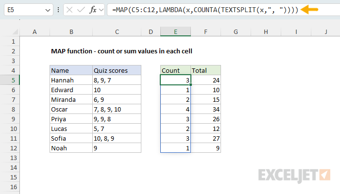
The TEXTSPLIT function splits each cell into its scores, and COUNTA counts them. In the second formula, the double negative (--) converts the scores, which are text after the split, to numbers, and SUM adds them up.

Why do we need MAP? TEXTSPLIT can't split a whole range: =TEXTSPLIT(C5:C12,", ") returns only the first score from each cell, because a separate result for each cell would be an array of arrays. MAP splits one cell at a time, and COUNTA or SUM reduces each split to one number, which is the single value MAP needs.

Get initials for a seating chart

MAP isn't limited to one column. Given a range with rows and columns, it runs the LAMBDA on every cell and returns a result with the same shape. In the worksheet below, the names in B5:D16 are a seating chart, and the goal is to show the same chart with initials. The formula in F5 is:

=MAP(B5:D16,LAMBDA(n,CONCAT(LEFT(TEXTSPLIT(n," ")))))

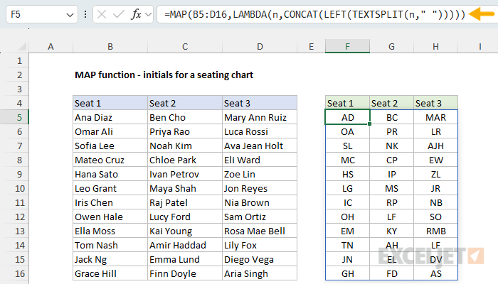
MAP passes each name to n, one at a time. TEXTSPLIT splits the name into words at each space, LEFT returns the first letter of each word, and CONCAT joins the letters into one text value. A name with a middle name, like "Mary Ann Ruiz", returns three initials. The results spill into F5:H16, in the same layout as the names: 12 rows and 3 columns.

This is the same pattern as the previous example: split each value, then combine the parts into one result. BYROW and BYCOL can't do this, because they run once per row or column, not once per cell. For more ways to shorten names, see Abbreviate names or words.

An empty seat returns #VALUE!, because TEXTSPLIT has nothing to split. To leave it blank, test for an empty cell first: =MAP(B5:D16,LAMBDA(n,IF(n="","",CONCAT(LEFT(TEXTSPLIT(n," ")))))).

Count visible rows with criteria

Counting or summing only visible rows is an interesting challenge, because Excel does not have a function that will return the visibility of a cell. The SUBTOTAL function can count or sum only the visible rows in a range. However, it returns one result for the whole range, and it can't apply criteria. We can work around this limitation with the MAP function to create a filter based on visibility.

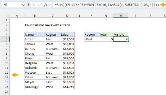
In the worksheet below, rows 7, 11, and 12 are hidden, and the goal is to count and sum the visible rows for the region in F5 ("West"). The formula in G5 looks like this:

=SUM((C5:C16=F5)*MAP(C5:C16,LAMBDA(c,SUBTOTAL(103,c))))

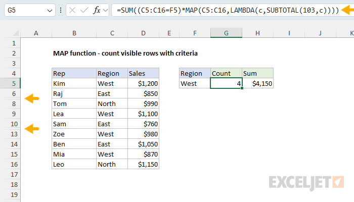
The expression C5:C16=F5 returns TRUE for each row in the West region:

{TRUE;FALSE;TRUE;FALSE;TRUE;FALSE;TRUE;FALSE;TRUE;FALSE;TRUE;FALSE}

This is one part of the required criteria. We only want to count values associated with the West region, which appear as TRUE in the array. The second part is cell visibility, which we handle with MAP:

MAP(C5:C16,LAMBDA(c,SUBTOTAL(103,c)))

Given a range, MAP passes each value to c (for cell) as a cell reference, which SUBTOTAL requires. Inside the LAMBDA, we check one cell at a time with SUBTOTAL(103,c). With function number 103, SUBTOTAL runs COUNTA and ignores hidden rows. Since we're working with one cell at a time, the result is 1 for a visible cell and 0 for a hidden one. MAP returns all 12 results in a single array like this:

{1;1;0;1;1;1;0;0;1;1;1;1}

We use this array as the visibility part of the criteria. Multiplying the two arrays keeps only the visible West rows, since TRUE and FALSE become 1 and 0 in math (see Boolean logic), and SUM adds up the result. The final array inside SUM looks like this:

=SUM({1;0;0;0;1;0;0;0;1;0;1;0}) // returns 4

In contrast, =COUNTIF(C5:C16,F5) returns 6, because COUNTIF counts the hidden rows too.

To sum the visible sales instead, use function number 109 (SUM, ignoring hidden rows) on the sales column. The formula in H5 is:

=SUM((C5:C16=F5)*MAP(D5:D16,LAMBDA(c,SUBTOTAL(109,c))))

With function numbers 103 and 109, SUBTOTAL ignores rows hidden by a filter and rows hidden by hand. For more on this problem, see Count visible rows with criteria.

Running count of each value

The MAP function is also an interesting way to create an expanding reference that spills automatically. In the worksheet below, the goal is to number each person's visits: Kim's first visit is 1, Kim's second visit is 2, and so on. With a standard formula copied down the column, you can use COUNTIF with an expanding range like this: =COUNTIF($B$5:B5,B5). MAP can do the same thing in one formula. The formula in D5 is:

=MAP(B5:B16,LAMBDA(c,COUNTIF(B5:c,c)))

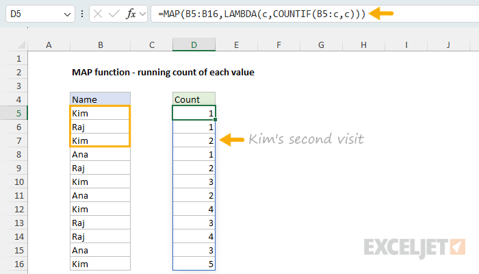
MAP passes each name as a cell reference, so B5:c is a real range from B5 down to the current cell. In row 7, B5:c is B5:B7, and COUNTIF counts 2 for "Kim". Each row's range is one cell longer than the last, just like the copied-down formula.

Note that this only works with a range. Given an array (for example, the result from FILTER), MAP passes each item as a value, not a reference, and B5:c returns #VALUE!.

Here are two variations on the same formula. The first adds the count to each name, and the second returns TRUE for each person's first visit, which is handy for flagging new visitors:

=MAP(B5:B16,LAMBDA(c,c&" "&COUNTIF(B5:c,c))) // returns "Kim 1", "Raj 1", "Kim 2", ...
=MAP(B5:B16,LAMBDA(c,COUNTIF(B5:c,c)=1)) // TRUE for each first visit

For a running total, use the SCAN function. For more on running counts, see Running count of occurrence in list.

Notes

• If the cells where the result should spill aren't empty, MAP returns #SPILL!. MAP also returns #SPILL! inside an Excel Table, because tables don't support spilling formulas.
• Arrays provided to MAP should be the same size. When they aren't, MAP pads the missing results with #N/A: =MAP({1,2,3},{10,20},LAMBDA(a,b,a+b)) returns {11,22,#N/A}. MAP also doesn't combine a row and a column into a grid the way ={1,2,3}+{10;20;30} does. For a grid, use MAKEARRAY.
• A value that is the same for every item, like a tax rate, belongs inside the LAMBDA, not in an array of its own. If you give MAP a single value as an extra array, it returns #VALUE!, and a single cell returns one result followed by #N/A.
• MAP accepts up to 253 arrays, since a LAMBDA can have at most 253 parameters. A LAMBDA with too many or too few parameters for the arrays returns #VALUE!.
• A LAMBDA that returns an array for an item causes MAP to return #CALC!. Reduce each result to one value with a function like TEXTJOIN, SUM, or COUNTA, as in List the matching words in each cell. To keep every value, see Return more than one result per row on the HSTACK page.
• An error in the data stays in its own result, and the other results are unaffected. But when an argument is an error, such as FILTER returning #CALC! when nothing matches, MAP returns that error.
• An empty cell comes through as empty, so ISBLANK(x) and x="" will both return TRUE. A LAMBDA that returns x shows 0 for an empty cell; use IF(x="","",x) to keep it blank. A formula that returns an empty string ("") isn't blank to ISBLANK, so x="" is the better test, since it catches both.
• Full-column references like MAP(B:B,...) return 1,048,576 results and #SPILL! in any cell below row 1. Use a range sized to the data, or a trim reference like B:.B.
• MAP runs the LAMBDA once per cell. BYROW and BYCOL run it once per row or column. To combine all the values into a single result, see REDUCE.
• MAP is available in Excel 2024+ and Excel 365, not Excel 2021.