BYCOL Function

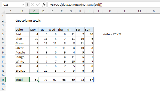
The BYCOL function applies a function to each column in array and returns one result per column in a single array. For example, if BYCOL is given a range with 10 columns, it returns an array of 10 results, one per column. The calculation performed on each column can be a built-in function like SUM or COUNT, or a LAMBDA function that operates on column values using custom logic.

BYCOL is especially useful in three situations:

1. To apply per-column logic that "collapses" an entire column of values into a single result. Anything with a conditional, threshold, or "all/any/none" test (for example, count values per column above 90, or flag columns where every value passes).
2. To generate a row of summary values or Booleans that can be used as an input to FILTER, SORTBY, INDEX, conditional formatting, or another calculation.
3. To perform per-column calculations on an array, not a range. When the input is an array produced by another formula (FILTER, VSTACK, TRIMRANGE, etc.), BYCOL gives you a convenient way to iterate over an array of unknown size and generate per-column calculations.

See below for specific examples.

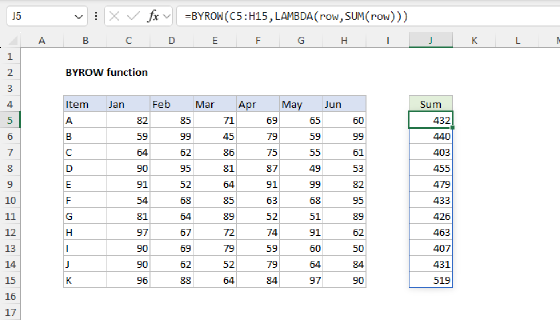
Note: BYCOL has two close siblings, BYROW and MAP. BYROW does the same thing across rows instead of columns, reducing each row to a single value. MAP applies a calculation to every cell rather than every row or column. Use MAP when you want to transform individual values. Use BYROW when you want to generate per-row calculations.

Key features

• Returns a single array with one result per column.
• Accepts any calculation that reduces a column to a single value (SUM, AVERAGE, MAX, TEXTJOIN, custom LAMBDA, etc.).
• Supports a concise "eta lambda" syntax for single-argument functions like SUM and MAX.
• The output can feed FILTER, SORTBY, INDEX, and other native array functions.
• Companion function: BYROW does the same across rows.
• Available in Excel 365 and Excel 2024.

Table of contents

• Basic usage
• Sum each column
• Count values per column that meet a condition
• Average each column ignoring zeros
• Flag columns with all, any, or none logic
• Column-level weighted average
• Sort columns by a calculated value
• Find column heading with the largest value
• Multiple calculations with VSTACK
• Notes

Basic usage

BYCOL takes two arguments: an array to process and a function to run on each column. The function can be written in two ways. The first way is as a long-form custom LAMBDA. This is the general form, and the one you'll see whenever the calculation needs custom logic:

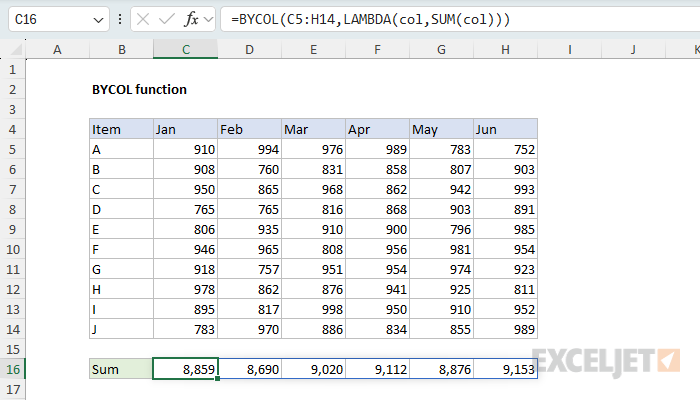
=BYCOL(array,LAMBDA(col,SUM(col)))
=BYCOL(array,LAMBDA(col,AVERAGE(IF(col<>0,col))))
=BYCOL(array,LAMBDA(col,MAX(col)-MIN(col)))

The second way is a short-form "eta lambda" syntax. Instead of wrapping the function in a LAMBDA, you provide just the function name. This works for single-argument functions like SUM, AVERAGE, MIN, MAX, COUNT, and COUNTA:

=BYCOL(array,SUM) // sum each column
=BYCOL(array,MAX) // max of each column
=BYCOL(array,AVERAGE) // average of each column
=BYCOL(array,COUNTA) // count of non-empty values

Note that the eta form can't be used when the calculation needs a comparison, a conditional, an extra reference, or any other logic. For those cases, use the long form.

The col name in the LAMBDA is arbitrary, and represents an entire column of data in the array provided. Use any name you like (c, x, values, etc.) as long as you're consistent inside the LAMBDA.

Sum each column

In the worksheet below, the goal is to sum the test scores in each subject column of the range C5:H14. The formula in C16 is:

=BYCOL(C5:H14,SUM)

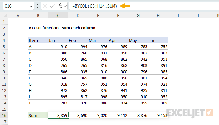
BYCOL processes all 6 subject columns at once and returns an array of 6 totals that spill into C16:H16. Notice we are using the short eta syntax above. The same pattern works for any single-argument aggregate:

=BYCOL(C5:H14,MAX) // max of each column
=BYCOL(C5:H14,MIN) // min of each column
=BYCOL(C5:H14,AVERAGE) // average of each column

Tip: If the source data will grow over time, wrap the range with the TRIMRANGE function or use the dot operator so BYCOL always gets just the used portion of the range: =BYCOL(C5:.N1000,SUM). The range becomes dynamic so results expand and contract with the data automatically.

Count values per column that meet a condition

BYCOL is useful when you want to count values per column that meet one or more specific conditions. This is where the eta syntax breaks down and the full custom LAMBDA syntax is required. In the worksheet below, the goal is to count the number of test scores in each subject above 90. The formula in C16 is:

=BYCOL(C5:H14,LAMBDA(col,SUM(--(col>90))))

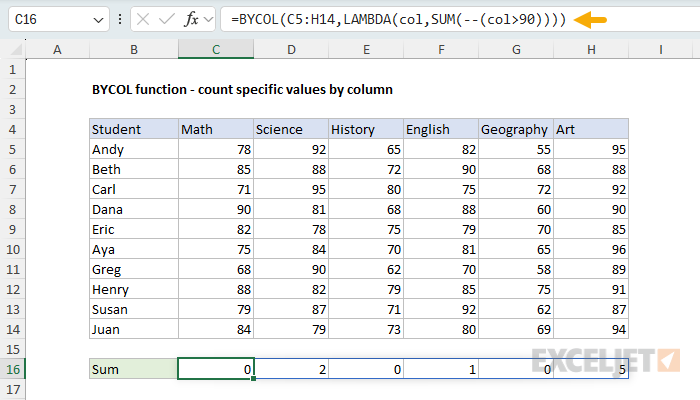
Working from the inside out, the logical expression col>90 returns an array of TRUE and FALSE values. The double negative (--) coerces the values to 1s and 0s, which SUM adds together to return the count. Because the calculation uses a comparison, the eta form won't work. We need a LAMBDA to hold the logical expression.

You might be tempted to use COUNTIF or COUNTIFS here, but the *IFS functions require a range, not an array, so they don't play nicely inside BYCOL. As a general rule, when you're working with arrays produced by other formulas, use Boolean logic instead of the *IFS family.

Average each column ignoring zeros

Zeros sometimes mean "no data" rather than "a real value of zero" (a student who missed an exam, a sensor that failed, a store that wasn't open, etc.). Averaging those zeros pulls the result down incorrectly. The BYCOL function gives you a clean way to exclude zeros when averaging column values. In the worksheet below, the goal is to calculate the average of each subject column while ignoring cells that contain 0 values. The formula in C16 is:

=BYCOL(C5:H13,LAMBDA(col,AVERAGE(IF(col<>0,col))))

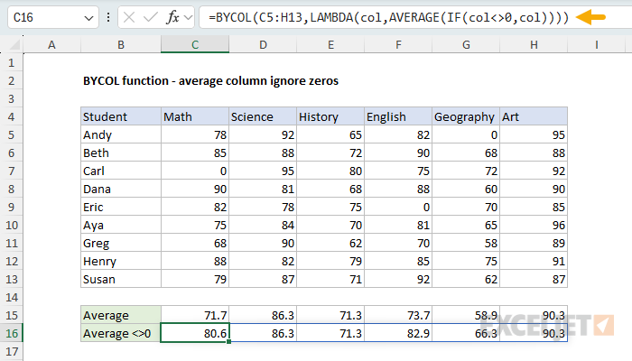
Inside the LAMBDA, the expression col<>0 returns TRUE for non-zero values and FALSE for zeros. The IF function passes only the non-zero values to AVERAGE; zero values become FALSE and are automatically ignored. The result is a per-column average that treats zeros as if they weren't there. For comparison, the formula in C15 (just above) does a simple average that includes all values, including zero:

=BYCOL(C5:H13,AVERAGE) // formula in C15 includes zero values

Flag columns with all, any, or none logic

One of BYCOL's most useful features is "collapsing" an entire column to a single TRUE or FALSE value. This lets you answer questions like "did every value pass?", "did any value hit the threshold?", or "did nothing fall below the limit?" for an entire column of values. In the worksheet below, each column holds the test scores for one subject across nine students. The formulas in C15, C16, and C17 evaluate each subject three different ways:

=BYCOL(C5:H13,LAMBDA(col,MIN(col)>=70)) // every student passed
=BYCOL(C5:H13,LAMBDA(col,MAX(col)>=95)) // anyone scored 95+
=BYCOL(C5:H13,LAMBDA(col,SUM(--(col<60))=0)) // nobody failed

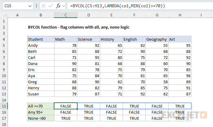
Each formula reduces a column of nine scores to a single TRUE or FALSE. The trick is picking the right aggregate function (MIN, MAX, SUM, etc.) to express the required logic:

• MIN(col)>=70: the smallest value passes, so all values must pass.
• MAX(col)>=95: the largest value hits the threshold, so at least one does.
• SUM(--(col<60))=0: none less than 60.

This pattern works any time you have a column-level rule that reduces to "yes" or "no". BYCOL generates the full row of results in a single formula, and that row can drive conditional formatting, highlight which subjects need attention, or feed into another function like FILTER (to filter by column).

While the worksheet above contains just nine students per subject, the same formulas would work just as well with a hundred.

Column-level weighted average

BYCOL's LAMBDA has access to more than just the col variable; you can reference other ranges or named ranges inside the LAMBDA. In the worksheet below, each column contains one student's scores across four scoring categories (homework, quizzes, midterm, final), and the weights appear in the named range weights (C5:C8). The goal is to calculate a weighted average for each student. The formula in D11 is:

=BYCOL(D5:H8,LAMBDA(col,SUMPRODUCT(col,weights)/SUM(weights)))

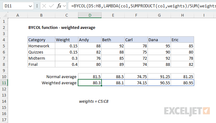
Inside the LAMBDA, the SUMPRODUCT function multiplies each column's values by the weights and sums the products. Dividing by the sum of weights normalizes the result so the weights don't have to add up to 1. BYCOL applies the calculation to all 5 students in a single formula and spills the weighted averages into D11:H11. For comparison, the formula in D10 calculates a normal (unweighted) average like this:

=BYCOL(D5:H8,AVERAGE) // formula in D10 averages without weights

This is a case where BYCOL replaces a copied-across helper formula. Without it, you'd write =SUMPRODUCT(D5:D8,weights)/SUM(weights) in D11 and copy across. That works fine, but with BYCOL, the calculation lives in one cell and can be adapted to extend the results dynamically by adding a dot operator like this:

=BYCOL(D5:.AZ8,LAMBDA(col,SUMPRODUCT(col,weights)/SUM(weights)))

The dot operator trims the range to the used portion of D5:AZ8, so AZ just sets a decent upper bound (up to 49 students) rather than a fixed end. Add or remove students and the formula adjusts automatically.

For more details on weighted averages, see Weighted average.

Sort columns by a calculated value

In this example, the goal is to sort monthly sales columns from highest total to lowest, so the top months appear on the left. The challenge is that the column total doesn't exist in the data. A traditional solution is to add a totals row, sort, then hide it. BYCOL makes that unnecessary. The formula in G4 is:

=SORTBY(C4:E9,BYCOL(C5:E9,SUM),-1)

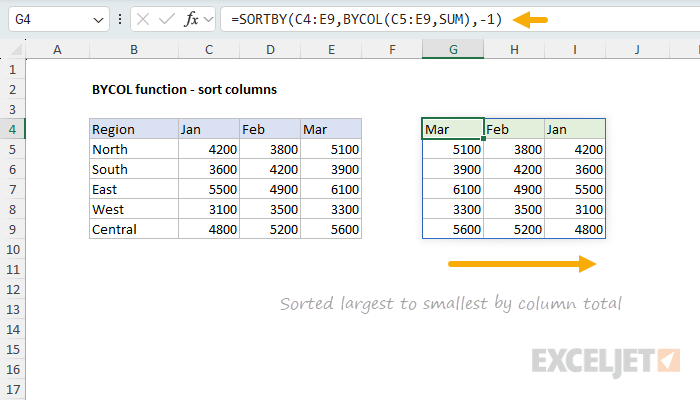
The first argument to SORTBY (C4:E9) deliberately includes the header row so each month's heading travels with its column when sorted. BYCOL operates on just the data rows (C5:E9) and returns a one-row array of column totals, which SORTBY uses as the by_array. Because that array is a row vector, SORTBY sorts the columns of the source array rather than the rows. The -1 sorts in descending order, so the month with the highest total appears first. The totals themselves never appear in the output; they're calculated on the fly, used only to drive the sort, and discarded.

The same pattern works for other calculations:

=SORTBY(data,BYCOL(data,LAMBDA(c,MAX(c)-MIN(c))),-1) // sort by volatility
=SORTBY(data,BYCOL(data,AVERAGE),1) // sort by column average, ascending

To extract the top n columns, wrap the result with the TAKE function:

=TAKE(SORTBY(C4:E9,BYCOL(C5:E9,SUM),-1),,2) // top 2 months by total

Find column heading with the largest value

When BYCOL returns a row of summary values, you can use XLOOKUP to look up the column heading associated with the largest result. In the worksheet below, the goal is to identify which subject has the highest class average. The formula in J5 is:

=LET(avgs,BYCOL(C5:H14,AVERAGE),XLOOKUP(MAX(avgs),avgs,C4:H4))

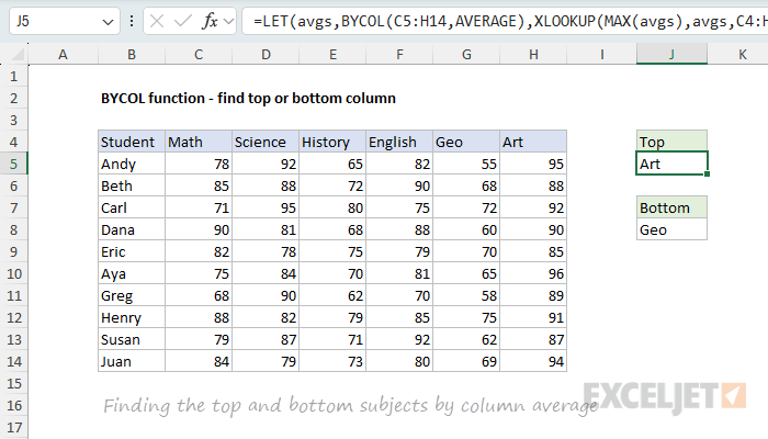
The LET function names the BYCOL result avgs so we don't have to calculate the same value twice. MAX returns the largest class average, and XLOOKUP looks that value up in avgs and returns the matching subject heading from C4:H4.

To find the subject with the lowest average score, just swap the MIN function for MAX. This is the formula in cell J8:

=LET(avgs,BYCOL(C5:H14,AVERAGE),XLOOKUP(MIN(avgs),avgs,C4:H4))

This is a useful pattern when the goal is "which column?" rather than "what's the value?": the strongest product, the best-performing region, the day with the most traffic, and so on.

Multiple calculations with VSTACK

BYCOL's function argument accepts a single calculation, but you can stack multiple calculations using the VSTACK function. In the worksheet below, BYCOL is configured to return the sum, max, min, and average for each column stacked vertically. The formula in C15 is:

=BYCOL(C5:H13,VSTACK(SUM,MAX,MIN,AVERAGE))

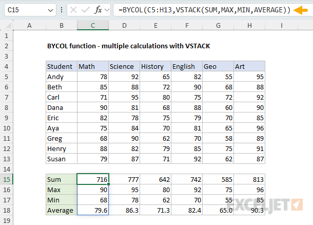
You can swap the functions inside VSTACK for any combination of aggregate results. Custom LAMBDAs work here too, as long as each one returns a single value.

Unfortunately, this formula will not spill across the full range of columns due to a current array of arrays limitation in Excel. You will get results for the first column only, and you'll need to copy the formula across manually to fill the rest. This is a known Excel limitation.

Notes

• BYCOL is available in Excel 365 and Excel 2024. Older versions don't support it.
• The calculation inside BYCOL should normally reduce each column to a single value. Returning an array per column will trigger the array of arrays limitation (see the VSTACK example).
• BYCOL processes all columns at once and returns a single spilled array. To send the output into another function like FILTER or SORTBY, use it directly; there's no need to write results to the sheet first.
• The col variable inside a LAMBDA is itself a one-column array, so it works in functions that accept arrays: SUM, AVERAGE, MAX, TEXTJOIN, MATCH, SUMPRODUCT, and so on.
• BYCOL can't see a column's position in the original data. If your calculation needs a column index, use MAKEARRAY or MAP with SEQUENCE instead.
• For row-by-row processing instead of column-by-column, use the BYROW function.