=REDUCE([initial_value], array, function)- initial_value - [optional] The initial value of the accumulator.
- array - The array to be reduced.
- function - The function or custom LAMBDA to apply.
Using the REDUCE function
The REDUCE function applies a custom LAMBDA function to each element in a given array and accumulates results to a single value. The REDUCE function is useful when you want to process each element in an array and return a single aggregated result. REDUCE is handy for creating custom calculations that Excel doesn't have built-in functions for, such as conditional sums, conditional counts, and other complex aggregations.
Like the SCAN function, REDUCE iterates over all elements in an array and performs a calculation on each element while updating the value of an accumulator. However, while SCAN returns an array of intermediate values, REDUCE returns a single final value.
Key features
- Reduce or aggregate values into a single result.
- Uses a custom LAMBDA function to apply calculations.
- Tracks the prior result of a calculation as an "accumulator".
- Complete control over how values accumulate.
- Good for conditional sums, counts, and other complex aggregations.
- Able to use logical functions like AND, OR, NOT, etc. to apply conditions.
- Can replace complex formulas with more readable and maintainable code.
REDUCE returns a single aggregated result after processing all elements in an array. To process an array and return all intermediate values, see the SCAN function. To process each element in an array individually and return an array of transformed results, see the MAP function.
Table of contents
- LAMBDA structure
- REDUCE for a basic conditional sum
- REDUCE for a conditional count
- REDUCE for conditional concatenation
- REDUCE to split comma-separated values
- REDUCE to extract unique words from a range
- REDUCE to extract and count unique words
- REDUCE to extract unique values case-sensitive
- REDUCE to remove unwanted text
- REDUCE to find and replace multiple values
LAMBDA structure
The REDUCE function takes three arguments: initial_value, array, and function. Initial_value is an optional initial seed value to use for the accumulator. Array is the array to reduce, and function is typically a custom LAMBDA function to apply to each value in the array. The structure of the LAMBDA used in REDUCE looks like this:
LAMBDA(a,v,calculation)
The first argument, a, is the accumulator. The accumulator begins as the initial_value provided to REDUCE and changes as the REDUCE function iterates over the elements in the array and applies a calculation. The v argument represents the value of each item in the array. The calculation is a formula that operates on the accumulator (a) and value (v). The result of the calculation defines the value of the accumulator for the next iteration, and the final result is the value of the accumulator after all elements have been processed. For example, in the formula below, REDUCE is used to sum all values in an array:
=REDUCE(0,{1,2,3,4,5},LAMBDA(a,v,a+v)) // returns 15
The initial_value is provided as zero, the array is hard-coded as the array constant {1,2,3,4,5}, and the calculation, LAMBDA(a,v,a+v), simply adds the accumulator and value. The table below shows how the accumulator value changes during each iteration as REDUCE processes the array {1,2,3,4,5} starting with an initial value of 0. Notice that the accumulator is updated with the result of the calculation at each iteration.
| Iteration | Value (v) | Accumulator (a) | Calculation | Result |
|---|---|---|---|---|
| Initial | - | 0 | - | - |
| 1 | 1 | 0 | 0 + 1 | 1 |
| 2 | 2 | 1 | 1 + 2 | 3 |
| 3 | 3 | 3 | 3 + 3 | 6 |
| 4 | 4 | 6 | 6 + 4 | 10 |
| 5 | 5 | 10 | 10 + 5 | 15 |
The final result returned by REDUCE is 15, which is the final value of the accumulator after all elements have been processed.
The REDUCE function always assigns the first argument of LAMBDA to the accumulator (a) and the second argument to the current value (v) from the array. This behavior is built into the function's design and cannot be changed. The names a and v are arbitrary, used to represent accumulator and value. You can use any names that make sense to you for a given use case.
As mentioned above, initial_value is optional. Although it does not appear in Excel's official documentation, it seems that if the initial value is omitted, it does not default to zero (0) or an empty string ("") as you might expect. Instead, REDUCE takes the first element of the array as the initial value, then iterates over the remaining elements of the array. In other words, if you omit the initial_value, Excel treats the first element of the array as the starting accumulator, and processing continues from the second element onward. To avoid confusion, it's a good idea to set the initial value explicitly. One possible exception is when using REDUCE with VSTACK to stack 1D arrays. In that case, using an empty string ("") for the initial value will result in an extra element in the final array, which you will need to remove later with the DROP function. Omitting the initial value avoids this additional step.
REDUCE for a basic conditional sum
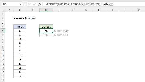
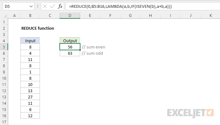
One way to use the REDUCE function is to create a conditional sum that uses custom logic that would be difficult with a built-in function like SUMIFS. In the worksheet shown below, we have a list of numbers in the range B5:B16, and we want to create a sum of the even numbers in the range. The formula in D5 looks like this:
=REDUCE(0,B5:B16,LAMBDA(a,v,IF(ISEVEN(v),a+v,a)))
Notice that we have provided an initial_value of zero (0) and the array is given as the range B5:B16. The LAMBDA calculation looks like this:
LAMBDA(a,v,IF(ISEVEN(v),a+v,a))
Inside the LAMBDA function, the a argument is the accumulator, and the v argument is the value. These values are provided by the REDUCE function. The IF function is used with the ISEVEN function to make the sum conditional. Values in the array are only added to the accumulator if they are even numbers. The REDUCE function iterates over all values in B5:B16. For each value v, it checks if it is even using ISEVEN. If it is even, it adds the value to the accumulator a. If it is not even, it keeps the accumulator unchanged. The final result is 40, the sum of the even numbers 2,4,6,10,6, and 12.
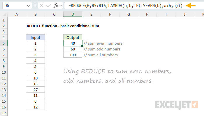
To calculate a conditional sum of odd numbers, we can simply swap ISEVEN for ISODD:
=REDUCE(0,B5:B16,LAMBDA(a,v,IF(ISODD(v),a+v,a)))
The only difference is that the ISODD function is used instead of ISEVEN. This formula works just like the formula in D5, but it sums the odd numbers instead of the even numbers. The final result is 60, the sum of the odd numbers 1,3,5,13,27, and 11.
Finally, to illustrate what the same formula looks like without any conditional logic, the formula in cell D7 sums all numbers in the range B5:B16 like this:
=REDUCE(0,B5:B16,LAMBDA(a,v,a+v))
Here, REDUCE iterates over the range B5:B16 and adds the accumulator and value unconditionally at each iteration. The final result is 100.
The reason this formula is difficult with the SUMIFS function is that SUMIFS requires a range for the criteria, but ISODD and ISEVEN will return an array of results.
REDUCE for a conditional count
REDUCE can also be used to create a conditional count using logic that is difficult with a built-in function like COUNTIFS. In the worksheet shown below, we have a list of values like A-67, B-75, A-71, and so on. The goal is to count values that begin with "A" and that are greater than 75. The formula in cell D5 looks like this:
=REDUCE(0,B5:B16,LAMBDA(a,v,IF(AND(TEXTBEFORE(v,"-")="a",VALUE(TEXTAFTER(v,"-"))>=75),a+1,a)))
Notice that we have provided an initial_value of zero (0), and the array is given as the range B5:B16. The LAMBDA calculation looks like this:
LAMBDA(a,v,IF(AND(TEXTBEFORE(v,"-")="a",VALUE(TEXTAFTER(v,"-"))>=75),a+1,a))
This example shows how the REDUCE function can be used with the AND function to apply two conditions to a value:
- The value must begin with A
- The number after the hyphen must be greater than or equal to 75
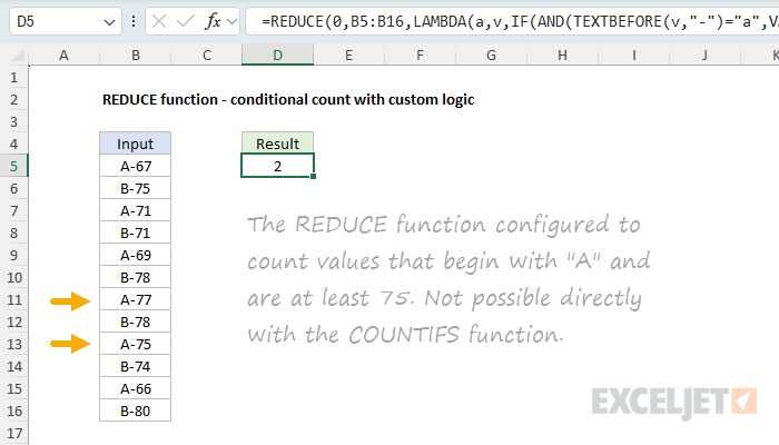
As always, the values for a and v are provided by the REDUCE function to the LAMBDA. The TEXTBEFORE function is used to get the text before the hyphen, and the TEXTAFTER function is used to get the text after the hyphen. The VALUE function is used to convert the text after the hyphen into a number. The IF function is used to check if the value meets the conditions defined by the AND function. If it does, the accumulator is incremented by 1. If it does not, the accumulator is returned unchanged. In this case, the final result is 2, since there are only two values that meet the conditions: A-77 and A-75.
This example illustrates how the REDUCE function can use logical functions like AND, OR, NOT, etc. to apply conditions to values. These functions aggregate an array of results into a single result, which causes trouble in array operations, but they work fine in REDUCE, since REDUCE deals with arrays one element at a time.
Notes: (1) The logic above could also be constructed with functions like LEFT, RIGHT, MID, etc. TEXTBEFORE and TEXTAFTER are handy because they'll work for any value that has a hyphen. (2) There are many ways to convert text to numbers in Excel. The VALUE function is one way, but you could also use a double negative
--, or add zero (0)+0.
REDUCE for conditional concatenation
REDUCE can also be used to concatenate values with conditional logic. In the worksheet below, the goal is to create a comma-separated list of names in column B that are greater than five characters long. The formula in D5 looks like this:
=REDUCE("",B5:B16,LAMBDA(a,v,IF(LEN(v)>5,IF(a="",v,a&", "&v),a)))
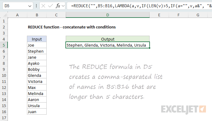
Notice that we have provided an initial_value of an empty string (""), and the array is given as the range B5:B16. The calculation inside the LAMBDA is:
LAMBDA(a,v,IF(LEN(v)>5,IF(a="",v,a&", "&v),a))
Starting with the initial value of an empty string (""), this formula iterates over each name in the range B5:B16 and uses the LEN function to check for names greater than five characters. When found, it adds the name to the accumulator with a comma and a space. If it is not, it keeps the accumulator unchanged. To avoid concatenating a comma to the start of the list, we need to do some extra checking with a second IF function:
IF(a="",v,a&", "&v)
This code only runs if we have found a name greater than five characters. If so, we check if the accumulator is an empty string. If it is, it means we have not yet found any names greater than 5 characters. In that case, we return just the value v to start the list. If the accumulator is not empty, it means we already have a name in our list, and we return a comma and a space followed by the new value.
This example nicely illustrates that the reduce function allows you full control over how the accumulator gets populated. However, I should note that there are different ways in Excel to solve this problem. You could, for example, use the FILTER function to isolate names that are greater than five characters and then use TEXTJOIN for concatenation.
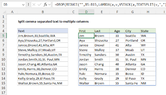
REDUCE to split comma-separated values
The REDUCE function works nicely with the VSTACK function to progressively build up an array of values. In the worksheet below, we have a list of comma-separated (CSV) values in column B, and the goal is to split each value in column B into the 5 columns to the right, as shown. The formula in D5 looks like this:
=DROP(REDUCE("",B5:B15,LAMBDA(a,v,VSTACK(a,TEXTSPLIT(v,",")))),1)
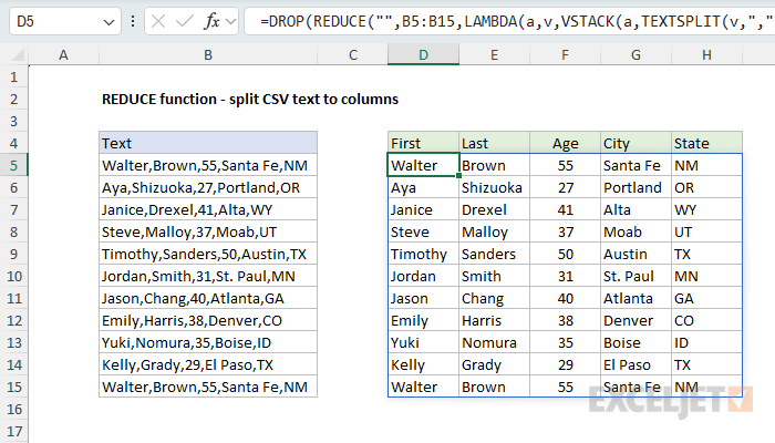
Notice that we have provided an initial_value of an empty string (""), and the array is given as the range B5:B16. The calculation inside the LAMBDA is:
LAMBDA(a,v,VSTACK(a,TEXTSPLIT(v,",")))
This formula works by iterating over each value in the range B5:B16 and splitting the value into an array of words using the TEXTSPLIT function. The VSTACK function is used to stack the results from TEXTSPLIT into a single array. The final result is an array of values in the range D5:H16. Notice we nest the REDUCE function inside the DROP function to remove the extra array created by setting the initial value to an empty string:
=DROP(REDUCE(...),1)
This formula works around an "array of arrays" limitation in Excel that prevents the TEXTSPLIT function from being used on a range of values. For a detailed explanation, see this article: Split comma-separated values to multiple columns.
REDUCE to extract unique words from a range
REDUCE can also be used with TEXTSPLIT to extract unique words from a range. In the worksheet below, the goal is to extract a list of unique words from the range B5:B16. The formula in D5 looks like this:
=UNIQUE(DROP(REDUCE("",B5:B16,LAMBDA(a,v,VSTACK(a,TEXTSPLIT(v,," ")))),1))
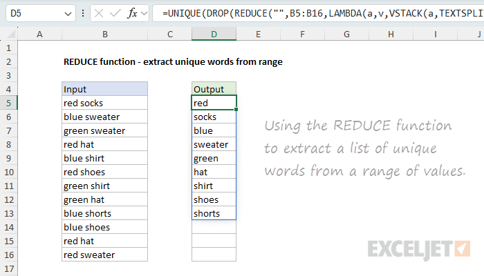
The initial value is an empty string (""), and the array is the range B5:B16. The calculation inside the LAMBDA is similar to the CSV example above, except we split text using a space (" ") as the delimiter instead of a comma:
LAMBDA(a,v,VSTACK(a,TEXTSPLIT(v,," ")))
The REDUCE function iterates over each value in B5:B16 and splits the text into separate words. Then it stacks the words vertically using the VSTACK function. When REDUCE is done, we have a single list of all words in the range. Next, the result from REDUCE is handed off to the DROP function, which removes the first row. This step is necessary because the initial value of an empty string ("") ends up in the final array. Finally, the result from DROP is passed to the UNIQUE function, which returns a list of unique words. This formula is a great example of how functions in Excel can be nested together:
=UNIQUE(DROP(REDUCE(...)),1))
Note: if you have inconsistent spacing between words, run the range through the TRIM function to remove extra spaces as a first step.
REDUCE to extract and count unique words
In the worksheet below, the goal is to extract a list of unique words from the range B5:B16 and generate a count for each word. This formula builds directly on the previous example. The formula in D5 looks like this:
=LET(
rng,B5:B16,
words,DROP(REDUCE("",rng,LAMBDA(a,v,VSTACK(a,TEXTSPLIT(v,," ")))),1),
GROUPBY(words,words,COUNTA,0,0,-2))
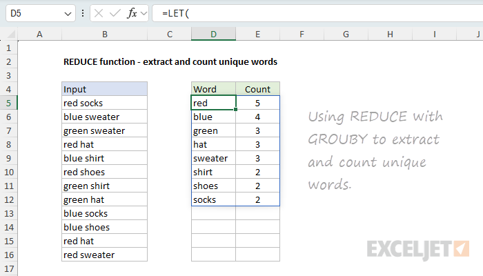
To keep things tidy, we use the LET function to create some variables. The variable rng is assigned the range B5:B16. The variable words is assigned the result from the REDUCE function, which is configured like the previous example, except we don't pass the result into UNIQUE. Instead, we pass the result into the GROUPBY function. The GROUPBY function works like a lightweight, formula-based pivot table. It automatically creates a list of unique words and, using the COUNTA function, generates a count for each word in one fell swoop.
Note: the GROUPBY function is a newer function with many configuration options. For a detailed guide, see this our article on the GROUPBY function.
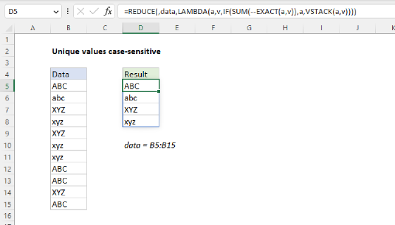
REDUCE to extract unique values case-sensitive
The REDUCE function can sometimes be used to work around difficult limitations in Excel. In the worksheet below, the goal is to extract a unique list of values from the range B5:B16, taking into account upper and lower case characters. This is a tricky problem in Excel because most built-in functions (including UNIQUE) are not case-sensitive. The formula in D5 avoids the UNIQUE function altogether and uses the EXACT function like this:
=SORT(REDUCE(,B5:B16,LAMBDA(a,v,IF(SUM(--EXACT(a,v)),a,VSTACK(a,v)))))
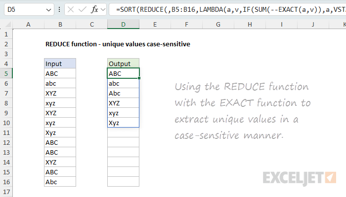
Notice that we are not providing an initial_value. This is a rare case where we omit the initial value altogether in order to avoid removing it later with the DROP function. This only works on one-dimensional arrays. The calculation inside the LAMBDA is:
LAMBDA(a,v,IF(SUM(--EXACT(a,v)),a,VSTACK(a,v)))
At a high level, this formula works by iterating over each value in the range B5:B16 and checking if the value v is equal to any value already in the accumulator a. If so, we return the accumulator unchanged. If not, we add the value v to the accumulator using the VSTACK function. The final result is an array of unique and case-sensitive values in the range. What makes the formula case-sensitive is the EXACT function, which is used together with the SUM function to check each value v against the accumulator a in this snippet, which is used as the logical test in the IF function:
SUM(--EXACT(a,v))
The EXACT function compares two text values in a case-sensitive manner. If the values are the same, it returns TRUE. If the values are different, it returns FALSE. If one of the values is an array (as with the accumulator in this example), the EXACT function will return an array of Booleans. In other words, each value v is tested against every value in the accumulator a and all results are returned. The double negative (--) coerces the Boolean values to 1s and 0s. The SUM function then adds up the 1s and 0s to give us a count. If the count is greater than 0, it means the value v is already in the accumulator a, so we return the accumulator unchanged. If the count is 0, it means the value v was not found in the accumulator a, so we add the value v to the accumulator using the VSTACK function. Finally, the result from REDUCE is passed to the SORT function, which sorts the unique values in ascending order.
For a more detailed explanation, see this article: Extract unique values case-sensitive.
REDUCE to remove unwanted text
In this example, the goal is to remove a list of unwanted characters from a range of text strings. This is a good example of how REDUCE can be used in ways that aren't immediately obvious. The text strings to process are in column B, and the characters to remove appear in the range F5:F10. The formula in D5 looks like this:
=TRIM(REDUCE(B5:B16,F5:F10,LAMBDA(a,v,SUBSTITUTE(a,v," "))))
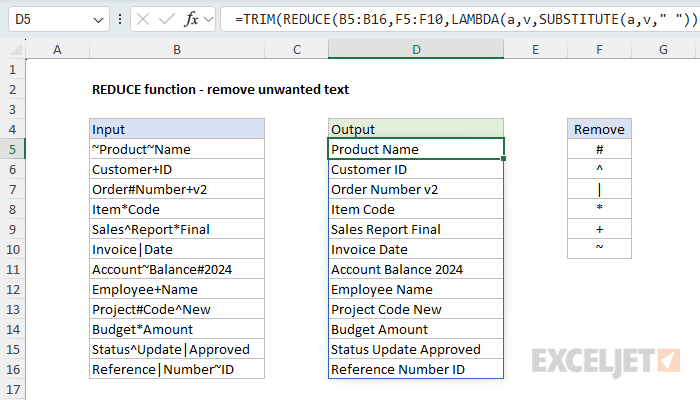
This is a pretty clever formula, and it is easy to get confused about how it works. The key is to look first at the initial value, which is provided as the range B5:B16. This is quite different from the above examples, where the values to process are typically provided as the array argument. Here, the values to process are provided as the initial_value, and the characters to remove are provided as the array. What this means is that we are actually calling the REDUCE function 12 times (through a built-in process called "lifting"), once for each value in the range B5:B16. Then, for each value in B5:B16, REDUCE iterates over the array of values in F5:F10 and applies a custom LAMBDA function like this:
LAMBDA(a,v,SUBSTITUTE(a,v," "))
The SUBSTITUTE function is used to replace the unwanted character with a space (" "). The accumulator a is an incoming value from B5:B16. The value v comes from F5:F10. Inside SUBSTITUTE, a is provided for text, v is provided for old_text, and a space (" ") is provided for new_text. At each iteration, the output from SUBSTITUTE a is used as the starting point for the next iteration. If the unwanted character is not found, SUBSTITUTE returns the value unchanged. When all unwanted values have been processed, REDUCE moves on to the next value in B5:B16. Finally, the result from REDUCE is passed to the TRIM function, which removes any extra spaces from the text strings.
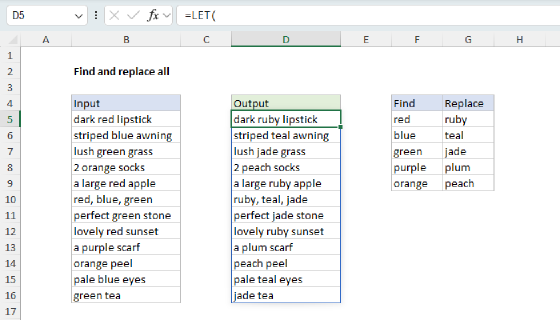
REDUCE to find and replace multiple values
In the previous example, we used the reduce function to replace multiple values with a single value. However, you may want to replace multiple values with multiple values in a "batch replace all" operation. In the worksheet below, the goal is to replace each of the "find" values in column F with the corresponding "replace" value in column G. The formula in D5 looks like this:
=LET(
    range,B5:B16,
    find,F5:F9,
    replace,G5:G9,
    ix, SEQUENCE(ROWS(find)),
    result, REDUCE(range,ix,LAMBDA(a,i,
        SUBSTITUTE(a,INDEX(find,i), INDEX(replace,i))
    )),
    TRIM(result)
)
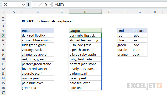
This formula is a bit more complex, but the setup is the same as the previous example: we provide source text in the range B5:B16 as the initial_value, then we provide an array that corresponds to the number of "find/replace" pairs in columns F and G as the array. The SEQUENCE function is used to create a sequence of numbers from 1 to the number of "find/replace" pairs in columns F and G. Since there are 5 rows in F5:F9, SEQUENCE returns the array {1;2;3;4;5}:
SEQUENCE(ROWS(find)) // returns {1;2;3;4;5}
This gives us an array that REDUCE can iterate over, and a list of indices that we can use to look up the corresponding "find" and "replace" values in columns F and G. As in the previous example, we use the lifting process to call the REDUCE function 12 times (once for each value in the range B5:B16). Then, for each value in B5:B16, REDUCE iterates over the array of values in F5:F9 and applies a custom LAMBDA function like this:
LAMBDA(a,i,SUBSTITUTE(a,INDEX(find,i), INDEX(replace,i)))
The SUBSTITUTE function is used to replace the "find" value with the "replace" value. The INDEX function is used to get the "find" and "replace" values from the corresponding columns. The i argument is the index of the current value in the array. The a argument is the accumulator, which is the current value in the range B5:B16. The result from SUBSTITUTE is used as the starting point for the next iteration. When all "find/replace" pairs have been processed, REDUCE moves on to the next value in B5:B16. Finally, the result from REDUCE is passed to the TRIM function, which removes any extra spaces from the text strings.
You can extend and customize the table of replacements as needed. If you need better control over word boundaries (i.e., you don't want to match "red" inside "bored", replace the SUBSTITUTE function with the REGEXEXTRACT function like this:
=LET(
    range,B5:B16,
    find,F5:F9,
    replace,G5:G9,
    ix,SEQUENCE(ROWS(find)),
    result,REDUCE(range,ix,LAMBDA(a,i,
        REGEXREPLACE(a,"\b"&INDEX(find,i)&"\b",INDEX(replace,i))
    )),
    TRIM(result)
)
If you are new to Regular Expressions (regex) in Excel, see our regex guide here.