=LET(name1, value1, [name2/value2], ..., result)- name1 - First name to assign. Must begin with a letter.
- value1 - The value or calculation to assign to name1.
- name2/value2 - [optional] Second name and value. Entered as a pair of arguments.
- result - A calculation that uses the named variables, or a variable previously defined. Must be the last argument.
Using the LET function
The LET function lets you define named variables in a formula. There are two primary reasons you might want to do this: (1) to improve performance by eliminating redundant calculations and (2) to make more complex formulas easier to read and write. Once a variable is named, it can be assigned a static value or a value based on a calculation. The formula can then refer to the variable by name as many times as needed, while the value of the variable is defined in one place only.
Variables are named and assigned values in pairs (name1, value1, name2, value2, etc.). LET can handle up to 126 name/value pairs, but only the first name/value pair is required. The final result is a calculation that uses the variables, or a variable previously calculated. The result from LET always appears as the last argument. The scope of each variable is limited to the LET formula itself: variables defined by LET cannot be seen or used by formulas in other cells.
The LET function is often combined with the LAMBDA function as a way to make a complex formula easier to use. The LAMBDA function provides a way to name a formula and reuse it in a worksheet like a custom function. Formulas based on LET and LAMBDA can be quite sophisticated, almost like a coding language, as seen in this formula to convert numbers into words.
Key benefits
The LET function provides three key benefits:
- Clarity - Named variables make complex formulas easier to read, write, and maintain.
- Simplification - Variables are named and defined in just one place, which reduces repetition and the errors that arise from having the same code in more than one place.
- Performance - Elimination of redundant code means less calculation time overall since expensive calculations only need to occur once.
Table of contents
- Basic examples
- Variable names
- Eliminate repetition
- List working days between dates
- Make a complex formula easier to read
- Line breaks and readability
- Split a full name into parts
- Round to significant figures
- Combine data from multiple worksheets
- Calculate income tax by bracket
- Build a search form with optional criteria
- Converting a formula to LET
- How to debug LET variables
- Best practices
- Notes
Basic examples
In its simplest form, the LET function takes three arguments: a name, a value to assign to the name, and a result that uses the name:
=LET(x,10,x+1) // returns 11
To define a second variable, add another name/value pair:
=LET(x,10,y,5,x+y) // returns 15
After x and y have been declared and assigned values, the calculation provided as the last argument returns a final result of 15. Variables can also be defined with a calculation, and later variables can refer to earlier variables:
=LET(x,10,y,x*2,x+y) // returns 30
Variables often get their values directly from the worksheet. For example, to multiply a price in cell B5 by a quantity in cell C5:
=LET(price,B5,qty,C5,price*qty) // price times quantity
In each case, the pattern is the same: names and values appear in pairs, and the final result is the last argument.
Variable names
The names used in LET must follow a few rules:
- Names must begin with a letter or an underscore (_).
- Names may contain letters, numbers, and the underscore character.
- Space characters and other punctuation symbols are not allowed.
- Names are not case-sensitive (
total=TOTAL). - Names must not conflict with Excel cell references like A1, etc.
The last point about cell references is a common gotcha. You can use names that contain numbers like "count1" and "count2", but a name like "ct1" will fail, because Excel interprets CT1 as a valid cell address:
=LET(count1,5,count1*2) // returns 10
=LET(ct1,5,ct1*2) // fails because ct1 is a valid reference
Note that you will not always receive a sensible error message if you try to use a variable name that is not allowed. If the name of the first variable is invalid, you do receive an error that makes sense:
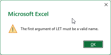
But if a later argument is a cell reference, you'll get a generic "There's a problem with this formula" error:
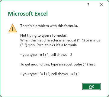
This error can be annoying because it's not clear what the problem is, and Excel will not let you enter the formula. Check your formula for names that conflict with cell references. Note that if you try to use a variable that you have not previously defined, you will get a standard #NAME? error. Make sure you have declared all names properly and check for typos. Finally, note that a LET variable will take priority over a named range with the same name inside the LET formula, so it is best to avoid names that overlap with existing named ranges.
Variable names are arbitrary and entirely under your control. You can name variables "x", "count", "date", etc. so long as the names are valid. I recommend you choose short names that make sense to you. A minimal name like "x" works fine in a short formula where the meaning is obvious, but descriptive names are more valuable as a formula grows. Name a variable for what it holds, not how it is calculated, and consider plural names for arrays ("dates") and singular names for single values ("date").
Eliminate repetition
A key benefit of the LET function is to remove redundancy. In the worksheet below, the goal is to look up a date with the XLOOKUP function and display a blank cell when the date is missing. The problem is that when XLOOKUP finds an empty cell, it returns a result that behaves like zero, which displays as "0-Jan-00" when formatted as a date (see cell H5). One fix is to test the result with the IF function, but a naive version of this formula requires two identical calls to XLOOKUP:
=IF(XLOOKUP(G5,B5:B16,D5:D16)="","",XLOOKUP(G5,B5:B16,D5:D16))
Translation: if the result is nothing, then return an empty string (""). With LET, we can run XLOOKUP just once, store the result, and reuse it later. The formula in cell H9 is:
=LET(x,XLOOKUP(G9,B5:B16,D5:D16),IF(x="","",x))
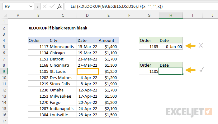
The first two arguments declare the variable x and assign the result from XLOOKUP to x. The final argument tests x: if the result is empty, the formula returns an empty string (""); otherwise it returns x. The logic is easier to follow, and XLOOKUP only runs one time. For more details, see XLOOKUP return blank if blank.
Programmers call this idea the DRY principle, short for "Don't Repeat Yourself": define each piece of logic in one place only. The idea is that when the same code appears in more than one place, the copies might drift apart as changes are made, and each copy is another chance for an error. The LET function allows you to implement this principle in Excel formulas. With LET, you can define things once, then reuse them by name as needed.
List working days between dates
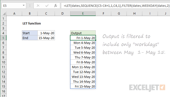
The LET function works well with dynamic array formulas, where the same array is often needed more than once. In the worksheet below, the goal is to list all working days (Monday through Friday) between the start date in cell C4 and the end date in cell C5. The formula in cell E5 is:
=LET(dates,SEQUENCE(C5-C4+1,1,C4,1),FILTER(dates,WEEKDAY(dates,2)<6))
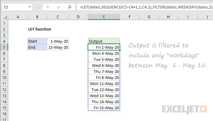
The SEQUENCE function generates all 15 dates between May 1, 2020 and May 15, 2020, and LET assigns the resulting array to the variable dates. The FILTER function then uses dates twice: once as the array to filter, and once inside the WEEKDAY function, which tests each date for weekdays. Only weekdays survive the filter, and the results spill into the range E5:E15. Without LET, SEQUENCE would need to appear twice in the formula with the same configuration. For a version of this formula that also excludes holidays, see List workdays between dates.
Make a complex formula easier to read
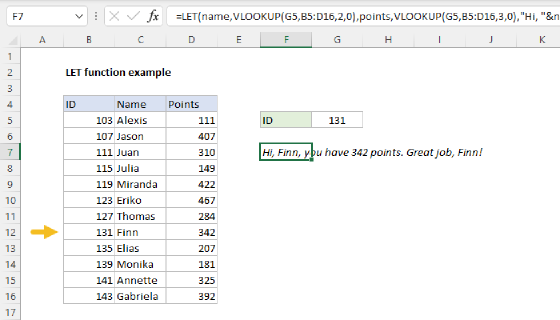
Named variables can make a formula much easier to understand, even when there is no performance benefit. In the worksheet below, the goal is to build a custom greeting for any ID entered in cell G5, using the name in column C and the points in column D. The formula in cell F7 is:
=LET(name,VLOOKUP(G5,B5:D16,2,0),points,VLOOKUP(G5,B5:D16,3,0),"Hi, "&name&", you have "&points&" points."&IF(points>300," Great job, "&name&"!",""))
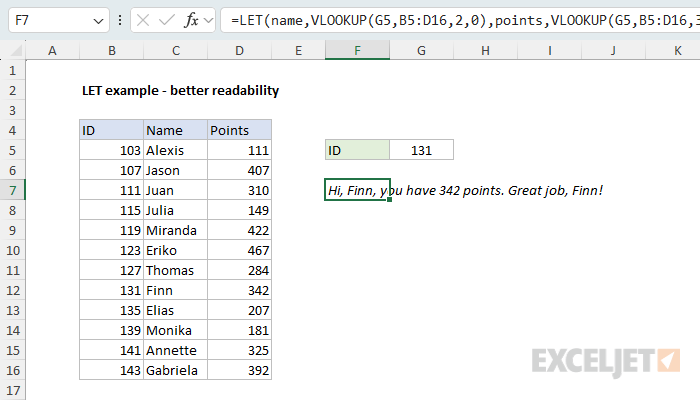
The VLOOKUP function is used to fetch name and points, and both variables are used twice in the message. Without LET, this formula would need four separate VLOOKUP calls, two of which would be exact duplicates. With LET, each lookup is defined once, and the concatenation at the end reads almost like a sentence. For a full walkthrough that builds this formula step by step, see Detailed LET function example.
Line breaks and readability
Formulas that use LET tend to get long, since each variable needs both a name and a value. To keep things readable, a common convention is to add line breaks so that each name/value pair sits on its own line, with the final result on the last line. Excel will automatically ignore extra white space in a formula. To add a line break inside a formula, use Alt+Enter. For example, here is the formula from the previous example with line breaks added to separate each variable:
=LET(
name,VLOOKUP(G5,B5:D16,2,0),
points,VLOOKUP(G5,B5:D16,3,0),
"Hi, "&name&", you have "&points&" points."&
IF(points>300," Great job, "&name&"!",""))
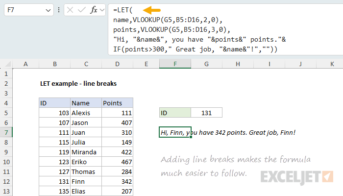
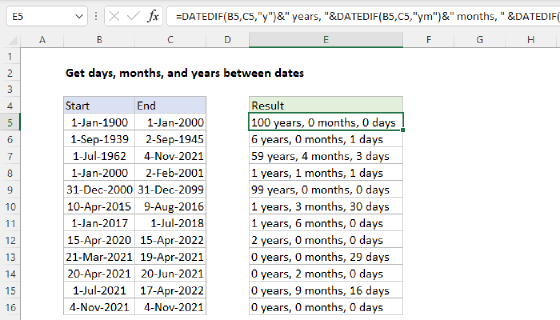
The trade-off with adding line breaks to a formula is that by default the formula bar shows just one line so a multi-line formula may appear cut off. To see the entire formula, expand the formula bar with the keyboard shortcut Control+Shift+U, or drag the bottom edge of the formula bar downward. For another example that builds up a more complex LET formula step by step, see Get days, months, and years between dates.
If you are used to writing short, elegant formulas in Excel, it can feel strange to purposely increase the length of a formula by adding line breaks. Personally, I think the improved readability is worth it.
Split a full name into parts
Variables in LET can build on each other to break a hard problem into simple steps. In the worksheet below, the goal is to split the full names in column B into first, middle, and last names. The challenge is that names have a variable number of parts: some have no middle name, and some have two middle names. The formula in cell D5, copied down, is:
=LET(
  parts,TEXTSPLIT(B5," "),
  count,COUNTA(parts),
  first,INDEX(parts,1),
  last,INDEX(parts,count),
  IFS(
    count=1,HSTACK(first,"",""),
    count=2,HSTACK(first,"",last),
    count>2,HSTACK(first,TEXTJOIN(" ",1,DROP(DROP(parts,,1),,-1)),last)
   )
)
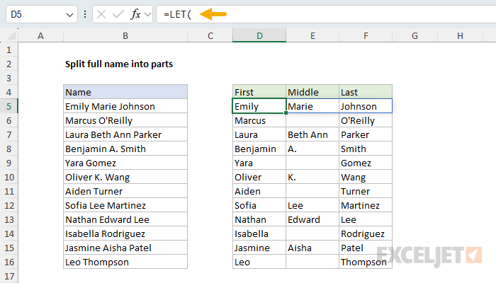
The TEXTSPLIT function splits each name into an array of parts, the COUNTA function counts the parts, and the INDEX function picks out first and last. Notice how each variable uses the variables defined before it. With the four variables in place, the IFS function handles the conditional logic for one, two, or many name parts. This is a formula that would be very difficult to write (and nearly impossible to read) without LET. For details, see Split full name into parts.
Round to significant figures
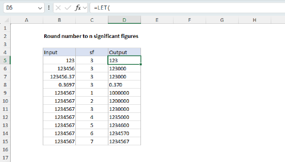
LET is also useful to simplify formulas that involve tricky math. In the worksheet below, the goal is to round the numbers in column B to the number of significant figures given in column C. The formula in cell D5, copied down, is:
=LET(
    number,B5,
    sf,C5,
    dp,sf-(1+INT(LOG10(ABS(number)))),
    rounded,ROUND(number,dp),
    IF(dp>0,TEXT(rounded,"0."&REPT("0",dp)),TEXT(rounded,"0")))
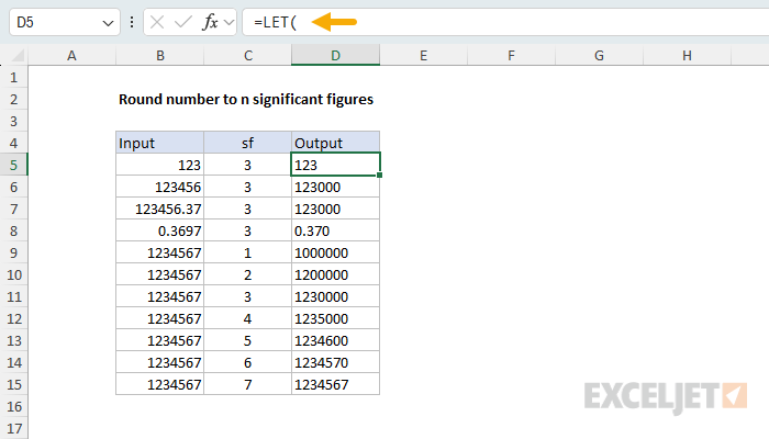
The first two variables, number and sf, simply pick up the inputs from the worksheet. The variable dp then calculates the decimal places needed with the LOG10 function, and rounded applies the ROUND function. Finally, the TEXT function formats the result to preserve trailing zeros. Each step has a name, so the logic is much easier to follow than the equivalent nested formula. For a full explanation of the math, see Round number to n significant figures.
Combine data from multiple worksheets
In the workbook below, the goal is to combine data from three worksheets into a single set of data without empty rows. The data on Sheet1, Sheet2, and Sheet3 has the same structure, and some rows in each range are empty. The formula in cell B5 on the summary sheet is:
=LET(data,VSTACK(Sheet1:Sheet3!B5:E16),FILTER(data,CHOOSECOLS(data,1)<>""))
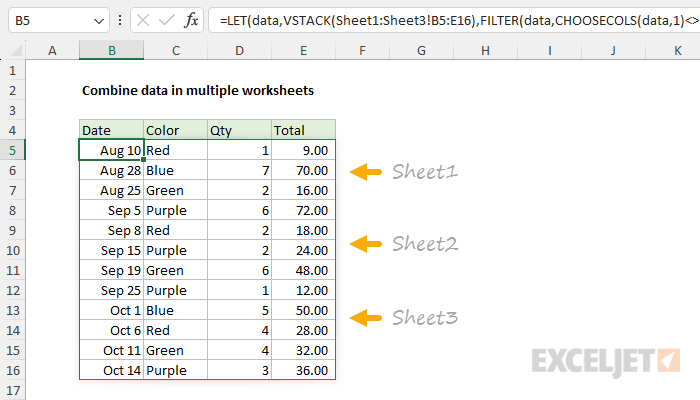
The VSTACK function uses a 3D reference to stack the range B5:E16 from all three sheets into a single array, which LET stores in the variable data. The FILTER function is then used to remove the empty rows that appear in some of the ranges. FILTER uses data twice: once as the array to filter, and once inside the CHOOSECOLS function, which tests the first column for empty cells. Because the combined data is stored in a variable, the (potentially expensive) VSTACK operation runs just once. For more details, see Combine data in multiple worksheets.
Calculate income tax by bracket
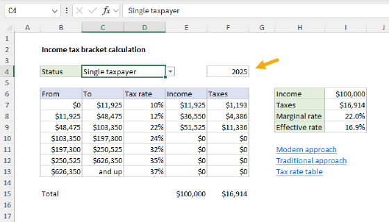
More advanced formulas may use LET to hold several intermediate arrays. In the worksheet below, the goal is to split the taxable income in cell I6 into the correct tax brackets, using only the upper limits in C7:C13. The formula in cell E7 is:
=LET(
income,I6,
upper,C7:C13,
lower,DROP(VSTACK(0,upper),-1),
IF(income<=lower,0,
IF(income>upper,upper-lower,income-lower))
)
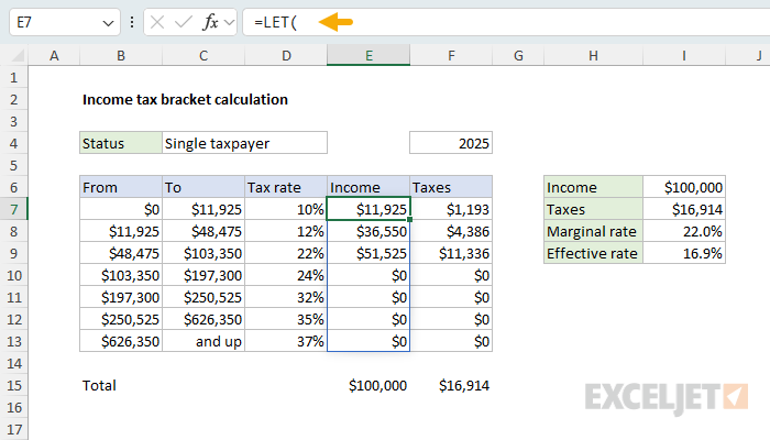
The variable income picks up the income from cell I6, and upper holds the upper limit of each bracket. The clever part is lower: the VSTACK function inserts a zero at the top of the upper limits, and the DROP function removes the last value, which shifts the array down one position to create the lower limits automatically. The nested IF function then compares the income to both arrays at once and returns the portion of income that falls into each bracket, which spills into E7:E13. One formula splits the income across all seven brackets. For a complete walkthrough, including tax calculations and a traditional formula alternative, see Income tax bracket calculation.
Build a search form with optional criteria
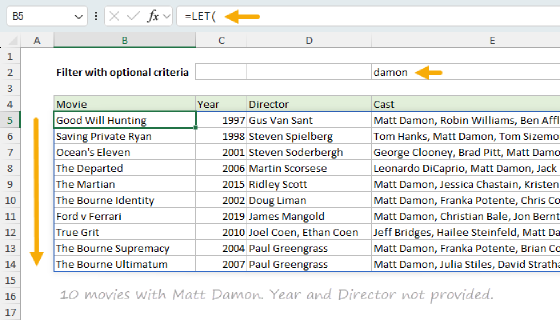
LET is a natural fit for formulas that combine several separate conditions, because each condition can be named and defined on its own line. In the worksheet below, the goal is to filter a list of 500 movies in an Excel Table named movies with three inputs: Year, Director, and Actor. Each input is optional: when an input is empty, the formula ignores that criteria. The formula in cell B5 is:
=LET(
  all,SEQUENCE(ROWS(movies))^0,
  year,IF(C2="",all,movies[Year]=C2),
  director,IF(D2="",all,ISNUMBER(SEARCH(D2,movies[Director]))),
  actor,IF(E2="",all,ISNUMBER(SEARCH(E2,movies[Cast]))),
  FILTER(movies,year*director*actor,"No match")
)
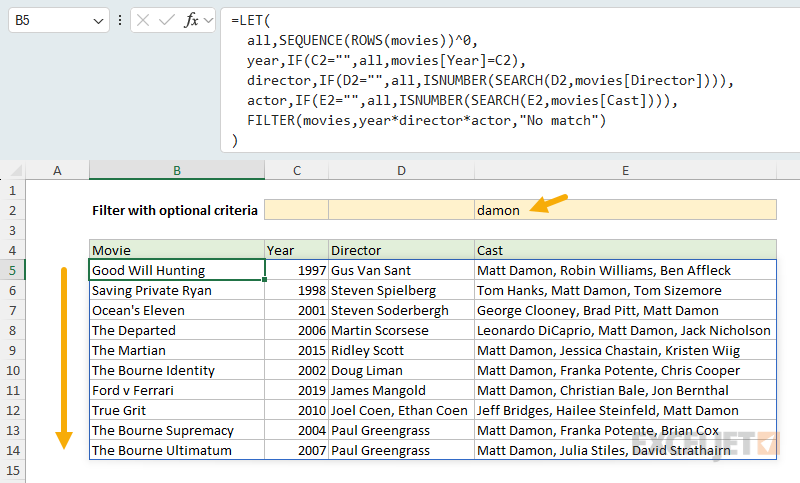
The variable all is an array of 1s, one for each row in the data, created with the SEQUENCE function. The variables year, director, and actor each test one input against one column, and return all when the input is empty. Since multiplying by 1 has no effect, an empty input effectively removes itself from the filter. Finally, the FILTER function multiplies the three arrays together and returns the matching records. Because each condition has a name, the logic is easy to follow, and new conditions can be added as needed by following the same pattern. For a full explanation, see FILTER with optional criteria.
Converting a formula to LET
Most LET formulas start out as regular formulas. When a formula becomes hard to read, or when you notice the same calculation appearing more than once, you can convert the formula to LET with a step-by-step process. As an example, the formula below checks whether the text in B5 contains only letters and numbers. This is a real-world formula used to apply data validation:
=AND(ISNUMBER(FIND(MID(LOWER(B5),SEQUENCE(LEN(B5)),1),"abcdefghijklmnopqrstuvwxyz0123456789")))
The formula works fine, but it has to be read from the inside out, the allowed characters are buried in the middle, and the input cell (B5) appears twice. To convert a formula like this to LET, follow these steps:
- Start with a working formula. Converting to LET should not change what a formula does, so begin with a formula that already returns correct results. Work with a copy, and check the result again after each step below.
- Wrap the formula in LET and define the inputs first. Inputs are the cell references the formula depends on. In this case, B5 appears twice, so we define
inputonce at the top and replace both references. - Name the settings. Settings are values that someone might want to change later. The string of allowed characters is an obvious example, so we assign the string to
allowed. Now the two things most likely to be edited sit together at the top of the formula. - Name the key calculation steps. Give each meaningful step a name that describes what the step returns. In this case, splitting the text into an array of characters becomes
chars. - Assign the final calculation to a variable named
result, and returnresultas the last argument.
Here is the final formula after conversion:
=LET(
input,B5,
allowed,"abcdefghijklmnopqrstuvwxyz0123456789",
chars,MID(LOWER(input),SEQUENCE(LEN(input)),1),
result,AND(ISNUMBER(FIND(chars,allowed))),
result
)
Notice that the order of the variables tells a story: here is the input, here is what is allowed, split the input into characters, then check every character. Each variable refers only to variables defined before it, and the formula reads from top to bottom like a series of steps, instead of from the inside out.
There is no need to name every expression in a formula. A variable earns its keep when it removes repetition (like input), names a cell reference, or gives a useful name to something otherwise unclear (like allowed). Naming trivial expressions just adds length. Finally, define a result variable with the last calculation, then return result on the last line. This seems redundant, but it makes the formula easier to troubleshoot, as explained in the next section.
For a complete explanation of the example above, see Data validation allow letters and numbers only. For another worked example of converting a formula, see Detailed LET function example.
How to debug LET variables
One challenge with the LET function is that intermediate values are hidden: there is no direct way to inspect the value assigned to a variable while the formula runs. You might expect Excel's built-in Evaluate Formula feature to help here, but it does not work well with LET. Evaluate Formula steps through a formula by substituting values into each expression, and with LET the substitutions quickly become long and hard to follow. You also can't use the keyboard shortcut F9 to inspect the value of a variable defined by LET; it will only return #NAME?.
The workaround is to temporarily change the result argument (the last argument) to return the variable you want to inspect. Because the result can be any variable previously defined, LET will simply output that variable to the worksheet. For example, to check the dates variable in the working days formula above, replace the final FILTER calculation with dates:
=LET(dates,SEQUENCE(C5-C4+1,1,C4,1),FILTER(dates,WEEKDAY(dates,2)<6)) // original
=LET(dates,SEQUENCE(C5-C4+1,1,C4,1),dates) // return dates to inspect
You can see the result below. This tells us the value of dates before we filter:
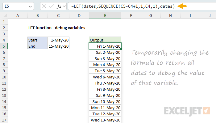
The second formula spills all 15 raw dates from SEQUENCE onto the worksheet, so you can confirm that the variable holds the values you expect. When a formula defines several variables, you can inspect each one the same way, working from the top down. This is a pain, since you have to edit the formula each time, but it is the most reliable way to see what is happening inside LET. Just remember to restore the original result when you are done. An easy way to do this is with the undo keyboard shortcut: Control+Z.
You can make this workflow easier by planning ahead: assign the final calculation to a variable named result, and end the formula by returning result. The working days formula would then look like this:
=LET(
dates,SEQUENCE(C5-C4+1,1,C4,1),
result,FILTER(dates,WEEKDAY(dates,2)<6),
result
)
The formula behaves exactly the same, but now the final calculation stays intact while you troubleshoot: to inspect a variable, edit only the last line (change result to dates), and type result again when you are done. It's a very unsophisticated approach, but it works well.
Microsoft offers a more capable formula editor called the Advanced Formula Environment (AFE), part of the free Excel Labs add-in. AFE provides a code-style editor with automatic formatting and support for inline comments, which makes large LET formulas easier to write and manage. You can see how I use AFE to handle a very large formula based on LET and LAMBDA in this example.
Best practices
Because LET is a relatively new function, best practices are not well established. In a way, LET introduces a classic programming problem (how to name things clearly) into the world of Excel formulas, and conventions will take time to develop and always involve personal preferences. That said, here are a few guidelines to use as a starting point:
- Use LET when a calculation is repeated. If the same expression appears more than once in a formula, define the expression as a variable so that it is calculated just once.
- Use LET to name confusing logic. A named calculation is easier to understand later.
- Don't use LET when it isn't needed. For short, simple formulas, LET just adds overhead. A formula like =B5*C5 does not benefit from variables.
- Name cell references at the top of the formula to make the formula easier to inspect and adapt. For example, the working days formula can be written like this:
=LET(
start,C4,
end,C5,
dates,SEQUENCE(end-start+1,1,start,1),
FILTER(dates,WEEKDAY(dates,2)<6))
- Variables can only refer to variables defined before them, so define values in the order they are needed. A useful general order is: inputs first, then settings a user might change (if relevant), then calculations.
- Don't name every expression. A variable earns its place when it removes repetition or makes the formula easier to understand. Naming trivial expressions just adds length.
- Assign the final calculation to a variable named
result, and returnresultas the last argument. This makes the formula easier to troubleshoot, as explained above. - Add line breaks to put each name/value pair on its own line, as explained above.
- Remember that LET requires Excel 2021+ or Excel 365.
If you have other suggestions for LET best practices, let me know.
Notes
- Defines named variables inside a formula, entered in name/value pairs
- Named variables can reduce or eliminate repetition
- The last argument to LET is always the final result
- Each value is calculated just once, which can improve performance
- Names are not case-sensitive.
- Variables defined by LET exist only inside the formula; other formulas cannot use them
- To reuse a value across many formulas, use a named range or the LAMBDA function.
- Variables can be defined based on earlier variables, not later variables
- Variables can hold static values, cell references, or calculated results, including arrays
- Available in Excel 2021+ and Excel 365