Summary
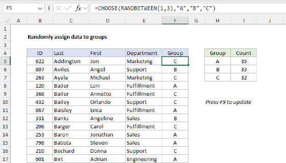
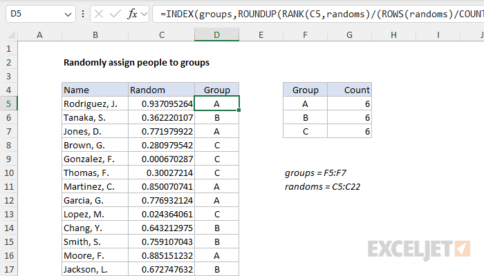
To randomly assign people to groups or teams of equal size, you can use a formula based on the RANK and ROUNDUP functions. In the example shown, the formula in D5 is:
=INDEX(groups,ROUNDUP(RANK(C5,randoms)/(ROWS(randoms)/COUNTA(groups)),0))
where groups (F5:F7) and randoms (C5:C22) are named ranges. As the formula is copied down, it returns a random group of "A", "B", or "C" on each row. In addition, the formula is configured to create groups of equal size.
Note: this problem can also be solved with a single Dynamic Array formula and no helper column. See below for details.
Generic formula
=INDEX(groups,ROUNDUP(RANK(C5,randoms)/(ROWS(randoms)/COUNTA(groups)),0))
Explanation
In this example, the goal is to randomly assign the names in column B to three groups of equal size. The group names are "A", "B", and "C", and these values appear in the named range groups (F5:F7). The solution should automatically count the number of groups to assign and attempt to generate the same count for each group. The worksheet shown contains 18 names, the final result should be that each group includes 6 random names from the list. The article below explains two approaches: (1) a traditional formula that depends on random values in a helper column, which will work in any version of Excel, and (2) a Dynamic Array formula that will return all random groups in one step without a helper column.
The solutions explained here are more complex because we are taking care to place the same number of people in each group when possible. To simply assign random groups without regard to size, see this page.
Basic approach
For both formulas explained below, the basic approach is the same and looks like this:
- Generate random numbers for each row
- Rank the random numbers
- Count groups and calculate the ideal group size
- Divide each rank by the group size
- Round the results up to the nearest whole number
- Use the whole number to fetch a group name with INDEX
The difference below is in the implementation. In older versions of Excel, we need to add a helper column that contains random numbers to the data, then use a formula that ranks each row according to the helper column. In the current version of Excel, we can use a single formula that generates all random numbers at once, and there is no need for a helper column.
Traditional formula
The traditional way to solve this problem in an older version of Excel is to use a helper column populated with random numbers with the RAND function, as seen in the worksheet above. In the worksheet shown, the random numbers appear in the range C5:C22 which is named "randoms" for convenience. To generate a full set of random values in one step, select the range C5:C22 and type =RAND() in the formula bar. Then use the shortcut control + enter to enter the formula in all cells at once.
Note: the RAND function will keep generating random values every time a change is made to the worksheet, so typically you will want to replace the results in column C with actual values using paste special to prevent changes after random values are assigned.
Assigning groups with INDEX
The formula used to assign random groups looks like this:
=INDEX(groups,ROUNDUP(RANK(C5,randoms)/(ROWS(randoms)/COUNTA(groups)),0))
At a high level, this formula uses the INDEX function to assign a group of "A", "B", or "C" to each name in the list. The generic pattern looks like this, where n is a number that corresponds to a group:
=INDEX(groups,n)
Because there are three groups total, the value for n needs to be between 1 and 3:
=INDEX(groups,1) // returns "A"
=INDEX(groups,2) // returns "B"
=INDEX(groups,3) // returns "C"
The hard part of the formula is generating a random number (n) for each row that will result in three groups of equal size. This is done in the snippet below, which makes up the bulk of the formula:
ROUNDUP(RANK(C5,randoms)/(ROWS(randoms)/COUNTA(groups)),0)
Working from the inside out, the first step is to assign a numeric rank to each random number with the RANK function:
RANK(C5,randoms)
RANK compares the number in cell C5 to all values in C5:C22 and returns its position relative to the other numbers in the range. The smallest number gets rank 1, the next smallest rank 2, and so on. Because there are 18 numbers in the list, RANK will generate a rank of 1-18. The next part of the formula calculates the optimal size for each group by dividing the total number of rows in the data by the number of groups to assign:
ROWS(randoms)/COUNTA(groups)
The ROWS function returns a count of rows (18), and the COUNTA function returns a count of groups (3). Simplifying, we have:
=ROWS(randoms)/COUNTA(groups)
=18/3
=6
The result is 6, which is the number of names that should be in each of the three groups. Next, the rank of each random number is divided by the number of names per group (6):
rank/6
For example, when a row is ranked 1st, the formula would return a value of 1/6, or 0.1667, when a row has a rank of 6, the formula returns 1/1, or 1, and so on. This is the mechanism by which the formula generates groups of equal size. The final step is to use the ROUNDUP function to round each number up to the next whole number, effectively dividing the ranked individuals into three equally sized groups based on their rank. The result from ROUNDUP is a random number between 1-3 (n) which is then used by INDEX to assign a group.
Dynamic Array formula
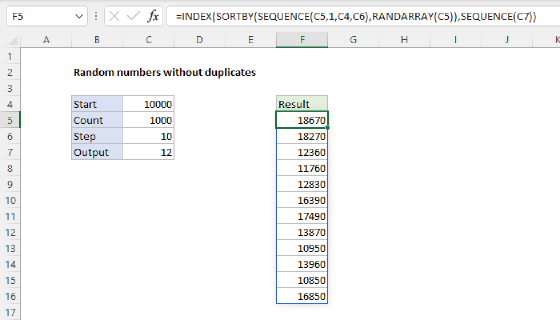
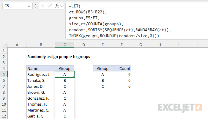
In Excel 2021 or later, dynamic array formulas allow a more sophisticated solution with an all-in-one formula that requires no helper columns. In the screen below, the formula in cell C5 is:
=LET(
ct,ROWS(B5:B22),
groups,E5:E7,
size,ct/COUNTA(groups),
randoms,SORTBY(SEQUENCE(ct),RANDARRAY(ct)),
INDEX(groups,ROUNDUP(randoms/size,0)))
This formula uses the LET function to create named variables within the formula, which reduces complexity and improves readability. In the first part of the formula, four variables are defined as follows:
- ct: The count of names, determined by ROWS(B5:B22).
- groups: The groups to be assigned in the range E5:E7.
- size: The size of each group, determined with ct/COUNTA(groups)
- randoms: A sorted list of random numbers created with SORTBY(SEQUENCE(ct), RANDARRAY(ct)).
The definition of randoms is the most interesting bit:
SORTBY(SEQUENCE(ct),RANDARRAY(ct))
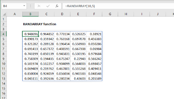
Since ct has been previously defined as 18, the SEQUENCE function creates an array of sequential numbers between 1 and 18. The RANDARRAY function creates an array of random numbers of the same size. Next, the SORTBY function sorts the sequence in the order of the random numbers, effectively shuffling the sequence. The result is the numbers 1 to 18 in a random order.
With the variables above in place, the last line in the formula generates the random groups like this:
INDEX(groups,ROUNDUP(randoms/size,0))
Like the original formula above, the basic pattern of this formula is:
=INDEX(groups,n)
where n is a random number between 1 and 3, corresponding to the three groups. The 18 individual values for n are calculated in one step like this:
ROUNDUP(randoms/size,0)
First, the numbers in randoms are divided by size to get a decimal number corresponding to a group. Then they handed off to the ROUNDUP function which rounds the numbers up to the nearest whole number. The result from ROUNDUP is an array that contains 18 numbers between 1 and 3. This array is returned directly to INDEX as the row_num argument, and INDEX returns the corresponding 18 groups in one step. The final result is that each group contains 6 random names from the list.
Conclusion
Although both formulas explained above work well, the dynamic array formula keeps all operations in a single cell. There is no need for a helper column. In addition, the LET function allows us to define variables that can be reused in the formula without recalculation, which makes the formula easier to read and more efficient. The result is a dynamic and efficient way to assign individuals to random groups of equal size with a single formula.