=RANK(number, ref, [order])- number - The number to rank.
- ref - A range that contains numbers to rank against.
- order - [optional] Whether to rank in ascending or descending order.
Using the RANK function
The RANK function returns the rank of a numeric value compared to a list of other numeric values. RANK can rank values from largest to smallest (i.e., the rank of highest test scores) and smallest to largest (i.e., the rank of fastest times in a race). You can use the RANK function to calculate the rank of each value in a dataset. RANK works fine with sorted or unsorted data — it is not necessary to sort the values in the list before using the RANK function.
Key Features
- Returns the rank of a single number against a list of other numbers
- Works with both ascending order (smallest = rank 1) and descending order (largest = rank 1)
- Does not require sorted data - works with data in any order
- Handles tied values by assigning the same rank to duplicates and skipping subsequent ranks
- Requires actual ranges - cannot use an array for the ref argument
- Compatibility function - Microsoft recommends using RANK.EQ or RANK.AVG instead
- Works in Excel 2003 and all later versions
Unlike most other Excel functions, RANK requires an actual range for the ref argument. If you try to use an array, Excel will not let you enter the formula.
Syntax
The basic syntax for RANK looks like this:
=RANK(number,ref,[order])
where number is the value you want to rank, ref is a range that contains numbers to rank against, and order is an optional argument for controlling ranking direction. By default, RANK will rank values in descending order and assign 1 to the largest value in the list. However, this behavior can be reversed using the optional order argument, as explained below.
Ranking in descending or ascending order
The rank function has two modes of operation, descending and ascending, which are controlled by the order argument. To rank values where the largest value is ranked number 1, set order to zero (0) or omit the argument altogether:
=RANK(A1,range) // rank descending (default)
=RANK(A1,range,0) // rank descending
To rank values where the smallest value should be 1, set order to 1:
=RANK(A1,range,1) // rank ascending
Set order to zero (0) when you want to rank something like top sales, where the largest sales number should rank #1, and set order to one (1) when you want to rank something like race results, where the shortest (fastest) time should rank #1.
Example - ranking test scores in descending order
In the worksheet below, the goal is to rank test scores. For test scores, the highest score should be assigned a rank of 1, so the RANK function is used in its default mode. The formula in cell D5 is:
=RANK(C5,$C$5:$C$12)
![]()
Notice that the range is provided as the absolute reference $C$5:$C$12 so that it won't change when the formula is copied down. The optional order argument is not provided, since RANK will assign 1 to the largest value by default.
Example - ranking race times in ascending order
In the example below, the goal is to rank race times. This is an example of where we want to assign a rank of 1 to the fastest time, which will be the smallest time. The formula in cell D5 is:
=RANK(C5,$C$5:$C$12,1)
Notice the range $C$5:$C$12 is absolute to prevent the reference from changing when the formula is copied down while the reference to C5 is relative so that it will change as the formula is copied down. Also, note that the optional order argument is provided as 1 to force RANK to rank the times in ascending order.
![]()
Ranking ties
Excel's RANK function handles ties in a specific manner: it assigns the same rank to both items. A tie occurs when two or more items in the data have the same value or, in other words, the data being ranked contains duplicates. For example, if a certain value has a rank of 3, and there are two instances of the value in the data, the RANK function will assign both instances a rank of 3. The next rank assigned will be 5, and no value will receive the rank of 4. The process looks like this:
- Ties are identified - When two or more values in the list are the same, they are considered tied. For example, if two students have a score of 91, they are in a tie.
- Ties are ranked - Excel assigns the same rank to the tied values. For instance, if two students are tied for the third-highest score, both will receive a rank of 3.
- The subsequent rank is skipped - After a tie, Excel skips the next rank(s). If two students are tied for third place, the next student (with a lower score) receives a rank of 5, not 3. The tie essentially absorbs the fourth rank.
You can see the result of this process in the worksheet below, where Aisha and Mia have a score of 91 and are both tied for third place. The RANK function assigns both a rank of 3 and the next rank, 4, is skipped.
![]()
If tied ranks are a problem, one workaround is to employ a tie-breaking strategy.
RANK versus RANK.EQ and RANK.AVG
Excel contains three functions for assigning rank: RANK, RANK.EQ, and RANK.AVG. RANK is the original ranking function in Excel. RANK.EQ and RANK.AVG were introduced in Excel 2010 as part of a broader effort by Microsoft to make Excel functions more consistent and intuitive. RANK and RANK.EQ are essentially the same function. There should be no cases where RANK and RANK.EQ return different results. RANK is still available in current versions of Excel for backward compatibility so that older spreadsheets that use RANK will still function as intended. The RANK.AVG function also assigns ranks to numeric values, but it provides a different behavior when there are tie values. Whereas RANK and RANK.EQ will assign tie values the same rank, the RANK.AVG function will assign tie values an average rank. For example, if two numbers are tied for third place, RANK.AVG will assign both numbers a rank of 3.5.
Recommendations
- The RANK function should continue to work fine in older worksheets. If you are updating an older worksheet, you could optionally replace RANK with RANK.EQ and get the same behavior and results.
- In new worksheets, Microsoft recommends RANK.EQ instead of RANK, since there is a possibility that RANK will be unsupported at some point in the future. Both RANK.EQ and RANK will return the same results and both will assign the same rank to tie values.
- If you specifically want an average rank for tie values in the data (i.e. duplicates) use the RANK.AVG function. This is the primary reason to use RANK.AVG since in other respects it works the same as RANK.EQ and RANK.
Notes
- The default for order is zero (0). If order is 0 or omitted, number is ranked against the numbers sorted in descending order: smaller numbers receive a higher rank value, and the largest value in a list will be ranked #1.
- If order is 1, number is ranked against the numbers sorted in ascending order: smaller numbers receive a lower rank value, and the smallest value in a list will be ranked #1.
- It is not necessary to sort the values in the list before using the RANK function.
- In the event of a tie (i.e. the list contains duplicates) RANK will assign the same rank value to each set of duplicates.
- Some documentation suggests ref can be an array, but in our testing, ref must be a range. Otherwise, Excel will display the "There's a problem with this formula" error dialog.