Summary
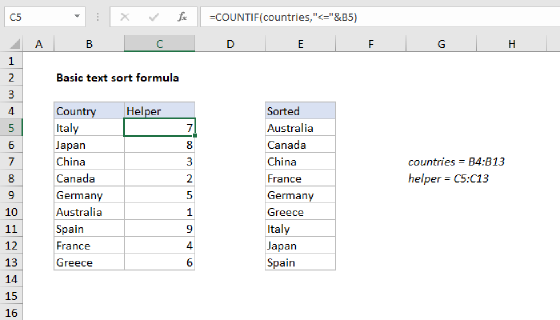
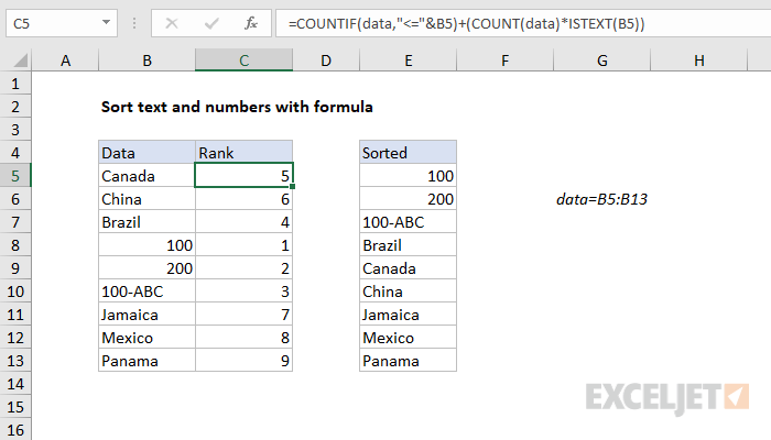
To dynamically sort data with both numbers and text in alphabetical order you can use a formula to generate a numeric rank in a helper column, then use INDEX and MATCH to display values based on rank. In the example shown the formula in C5 is :
=COUNTIF(data,"<="&B5)+(COUNT(data)*ISTEXT(B5))
where "data" is the named range B5:B13.
Generic formula
=COUNTIF(data,"<="&A1)+(COUNT(data)*ISTEXT(A1))
Explanation
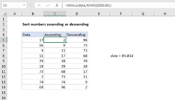
This formula first generates a rank value using an expression based on COUNTIF:
=COUNTIF(data,"<="&B5)
which is explained in more detail here. If the data contains all text values, or all numeric values, the rank will be correct. However, if the data includes both text and numbers, we need to "shift" the rank of all text values to account for the numeric values. This is done with the second part of the formula here:
+(COUNT(data)*ISTEXT(B7))
Here, we use the COUNT function to get a count of numeric values in the data, then multiply the result by the logical result of ISTEXT, which tests if the value is text and returns either TRUE or FALSE. This effectively cancels out the COUNT result when we are working with a number in the current row.
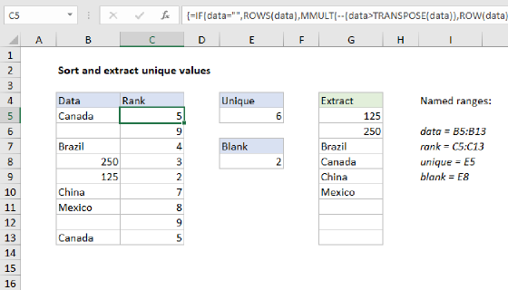
Handling duplicates
If data contains duplicates, the formula can be altered as shown below to assign a sequential rank to values that appear more than once:
=COUNTIF(data,"<"&B5)+(COUNT(data)*ISTEXT(B5))+COUNTIF($B$5:B5,B5)
This version adjusts the logic of the initial COUNTIF function, and adds another COUNTIF with an expanding reference to increment duplicates.
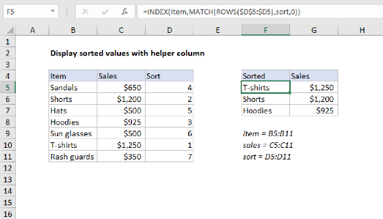
Display sorted values
To retrieve and display values sorted values in alphabetical order using the calculated rank value, E5 contains the following INDEX and MATCH formula:
=INDEX(data,MATCH(ROWS($E$5:E5),rank,0))
where "data" is the named range B5:B13, and "rank" is the named range C5:C13.
For more information about how this formula works, see the example here.
Dealing with blanks
Empty cells will generate a rank of zero. Assuming you want to ignore empty cells, this works fine because the INDEX and MATCH formula above begins at 1. However, you will see #N/A errors at the end of sorted values, one for each empty cell. An easy way to handle this is to wrap the INDEX and MATCH formula in IFERROR like this:
=IFERROR(INDEX(data,MATCH(ROWS($E$5:E5),rank,0)),"")