Random sort formula

To randomly sort existing values with a formula, you can use an INDEX and MATCH formula together with helper columns as shown in the screenshot. In the example shown, the formula in E5 is:

=INDEX(names,MATCH(ROWS($D$5:$D5),sort,0))

where "names" is the named range B5:B11, "rand" is the named range C5:C11, and "sort" is the named range D5:D11.

Note: If you are using a current version of Excel, this formula based on SORTBY and RANDARRAY is a better approach

Explanation

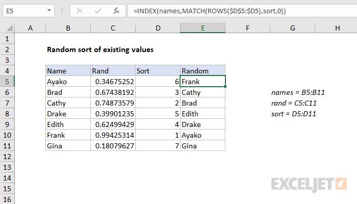
This formula depends on two helper columns. The first helper column holds random values created with the RAND() function. The formula in C5, copied down is:

=RAND()

The RAND function generates a random value at each row.

Note: RAND is a volatile function and will generate new values with each worksheet change.

The second helper column holds the numbers used to sort data, generated with a formula. The formula in D5 is:

=RANK(C5,rand)+COUNTIF($C$5:C5,C5)-1

See this page for an explanation of this formula.

The formula in E5 is:

=INDEX(names,MATCH(ROWS($D$5:$D5),sort,0))

Here, the INDEX function is used to retrieve values in the named range "names", using the sort values in the named range "sort". The actual work of figuring out what value to retrieve is done my the MATCH function in this snippet:

MATCH(ROWS($D$5:$D5),sort,0)

Inside MATCH, the ROWS function is given an expanding range as the lookup value, which begins as one cell, and expands as the formula is copied down the column. This increments the lookup value, starting at 1 and continuing to 7. MATCH then returns the position of the lookup value in the list.

The position is fed to INDEX as the row number, and INDEX retrieves the name at that position.