Display sorted values with helper column

To retrieve and display values sorted with a helper column, you can use an INDEX and MATCH formula, with a little help from the ROWS function. In the example shown, the formula in F5 is:

=INDEX(sales,MATCH(ROWS($D$5:$D5),sort,0))

which displays first item, based on the index provided in the helper column. The same approach is used to display associated sales in column G. For convenience, the worksheet contains the following named ranges: item = B5:B11, sales = C5:C11, sort = D5:D11.

In Excel 2021 and later, a better approach is to use the FILTER function. See this page for details.

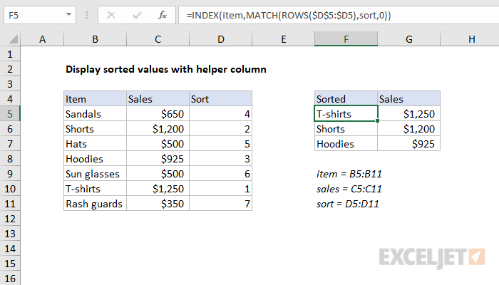
Explanation

This formula relies on a helper column that already contains a sequential list of numbers to represent an established sort order. The numbers in the helper column are independent of the operation of this formula. As long as the sequence is continuous, it can represent an ascending or descending sort, or even an arbitrary sort. In most cases, values will come from a formula.

At the core, this is a simple INDEX and MATCH formula, where INDEX retrieves a value based on a specified row number:

=INDEX(item,row)

The trick is that the row is calculated with the MATCH function based on values in the sort column:

MATCH(ROWS($D$5:$D5),sort,0)

The lookup value in MATCH is generated with the ROWS function and an expanding reference. In row 5 of the worksheet, the range includes one cell and ROWS returns 1. In row 6, the range includes two cells and ROWS returns 2, and so on.

The array is the named range "sort" (D5:D11). At each row, MATCH locates the lookup value and returns the position of that row number in the original data.

Since we want an exact match, the third argument, match type, is supplied as zero.

The value returned by MATCH feeds into the INDEX function as the row number, and INDEX returns the item at that position in the original data.