Random sort

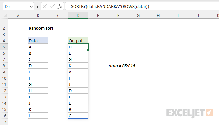
In this example, the goal is to perform a random sort of the data in B5:B16 with a formula. This can be done with the SORTBY function and the RANDARRAY function.

SORTBY function

The SORTBY function sorts provided values by one or more "sort by" arrays. The sort by arrays make it possible to sort data in a completely custom manner. The main requirement of the sort by array(s) is that they have dimensions that are compatible with the data being sorted. In this example, the named range data (B5:B16) holds the first 12 letters of the alphabet. That means we need a sort by array that contains 12 values. For example, we can sort the values in data in reverse order with a hardcoded array constant like this:

=SORTBY(data,{12;11;10;9;8;7;6;5;4;3;2;1})

The semicolons in the array used for sorting indicate a vertical array in rows, the same as the source data. To generate a random array of numbers to sort with, we need another function.

RANDARRAY function

The RANDARRAY function generates an array of random numbers between two values. The size or the array is determined by rows and columns arguments. To generate 12 random numbers to sort with, we can use the RANDARRAY function together with the ROWS function like this:

RANDARRAY(ROWS(data))

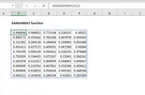
ROWS returns the number of rows in data, which in this case is 12. This number goes into the RANDARRAY function as the rows argument, and RANDARRAY returns an array of 12 decimal values like this:

{0.489071793902109;0.380639786424253;0.12859884623431;0.520000510523814;0.638866975537127;0.105109233209619;0.219291392470457;0.938867459800217;0.782387454565537;0.915924172473614;0.73975376365456;0.50617850806796}

Note: The array above is only an example. Because RANDARRAY generates a new set of random values with every worksheet change, it is difficult to capture the exact values used to sort the array.

Final formula

Bringing the pieces explained above together, the final formula used in D5 is:

=SORTBY(data,RANDARRAY(ROWS(data)))

ROWS provides a count of rows to RANDARRAY, which generates a random array of 12 decimal numbers. This array is returned directly to the SORTBY function as the by_array1 argument. SORTBY uses the random values to sort the data, and returns the 12 letters into a spill range starting in D5.

Note: RANDARRAY is a volatile function and will recalculate every time the worksheet is changed, causing values to be resorted. To stop values from sorting automatically, you can copy the formulas, then use Paste Special > Values to convert formulas to static values.