Summary
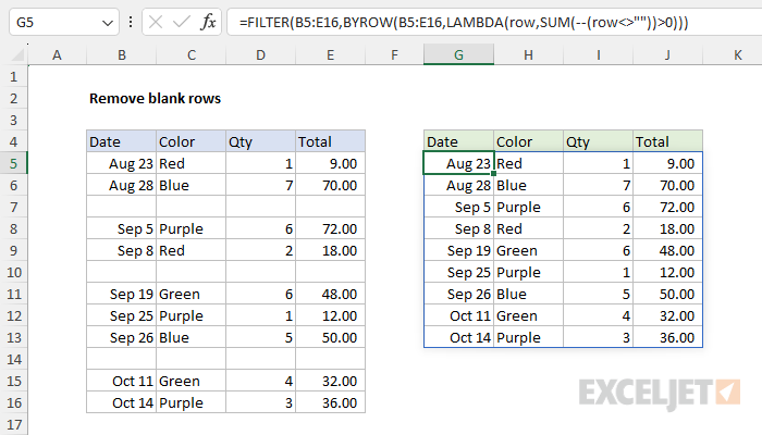
To remove blank/empty rows from a range, you can use a formula based on the FILTER function and the BYROW function. In the worksheet shown, the formula in cell G5 is:
=FILTER(B5:E16,BYROW(B5:E16,LAMBDA(row,SUM(--(row<>""))>0)))
When the formula is entered in cell G5, the FILTER function uses the result from the BYROW function to return only non-empty rows from the range B5:E16.
Generic formula
=FILTER(data,BYROW(data,LAMBDA(row,SUM(--(row<>""))<>0)))
Explanation
In this example, the goal is to remove empty rows from a range with a formula. One approach is to use the BYROW function to identify all non-empty rows in the range and pass this result into the FILTER function as the include argument. This is the approach used in the worksheet shown, where the formula in cell G5 is:
=FILTER(B5:E16,BYROW(B5:E16,LAMBDA(row,SUM(--(row<>""))>0)))
Working from the inside out, the BYROW function is used to check for non-blank rows like this:
BYROW(B5:E16,LAMBDA(row,SUM(--(row<>""))>0))
The purpose of BYROW is to process data in an array or range in a "by row" fashion. At each row, BYROW applies a custom LAMBDA function that contains the calculation needed to achieve the desired result. In this case, we want to identify non-blank rows. In other words, we want to check for rows that contain content in any cell. This is done in the following snippet:
LAMBDA(row,SUM(--(row<>""))>0)
The BYROW function delivers the range B5:E16 row-by-row to the LAMBDA above as the row argument. The LAMBDA then runs this calculation on each row:
SUM(--(row<>""))>0
The <> operator means "not equal to", so <>"" means "not empty". The result is an array of TRUE and FALSE values. In row 5, the result is an array like this:
=SUM(--({TRUE,TRUE,TRUE,TRUE}))>0
Next, the double negative (--) above converts TRUE to 1 and FALSE to 0:
=SUM({1,1,1,1})>0 // returns TRUE
The SUM function then returns 4, and the expression returns TRUE since 4 is greater than 0. Each row is processed in the same way, and BYROW returns all results in a single array like this:
{TRUE;TRUE;FALSE;TRUE;TRUE;FALSE;TRUE;TRUE;TRUE;FALSE;TRUE;TRUE}
Notice the array contains 12 results because the original range contains 12 rows. In this array, TRUE indicates non-empty rows and FALSE indicates empty rows. The array is returned directly to the FILTER function as the include argument:
=FILTER(B5:E16,{TRUE;TRUE;FALSE;TRUE;TRUE;FALSE;TRUE;TRUE;TRUE;FALSE;TRUE;TRUE})
FILTER returns the 9 rows that correspond to TRUE as a final result.
Simple option
The formula above is more complex because it tests every cell in a row to make sure it is empty. If you only need to test a single column to determine if a row is blank you can use a simpler formula like this:
FILTER(range,CHOOSECOLS(range,1)<>"")
In this formula, we use the FILTER formula as before. However, for the include argument we use the CHOOSECOLS function instead of BYROW:
CHOOSECOLS(range,1)<>"" // column 1 only
CHOOSECOLS runs first and extracts just the first column from the range. Then we simply test each cell in the column with <>"". Because each cell corresponds to a row, the result is a single array of TRUE and FALSE values that are used to filter the range. Adapting this formula to the example above, we have:
=FILTER(B5:E16,CHOOSECOLS(B5:E16,1)<>"")
After CHOOSECOLS is evaluated, we have the following:
=FILTER(B5:E16,{TRUE;TRUE;FALSE;TRUE;TRUE;FALSE;TRUE;TRUE;TRUE;FALSE;TRUE;TRUE})
The final result is the same as the FILTER + BYROW formula above. Note however that we are only testing column 1, so rows that contain data in other columns will be discarded.
More details
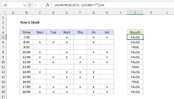
- To simply identify blank and non-blank rows, see: Row is blank.
- For more on the Boolean logic used above, see Boolean operations in array formulas.