Summary
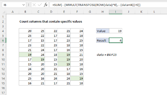
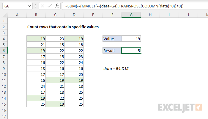
To count rows that contain specific values, you can use a formula based on the MMULT, TRANSPOSE, COLUMN, and SUM functions. In the example shown, the formula in G6 is:
=SUM(--(MMULT(--(data=G4),TRANSPOSE(COLUMN(data)^0))>0))
where data is the named range B4:D15. The result is 5, the number of rows that contain the number 19.
Note: this is an array formula and must be entered with control shift enter in Legacy Excel. See below for a formula that performs the same task with the newer BYROW function.
Generic formula
=SUM(--(MMULT(--(criteria),TRANSPOSE(COLUMN(data)))>0))
Explanation
In this example, the goal is to count the number of rows in the data that contain the value in cell G4, which is 19. The main challenge in this problem is that the value might appear in any column, and might appear more than once in the same row. If we wanted to simply count the total number of times a value appeared in a range, we could use the COUNTIF function. But we need a more advanced formula to count rows that may contain multiple instances of the value. The explanation below reviews two options: one based on the MMULT function, and one based on the newer BYROW function.
Background study
MMULT option
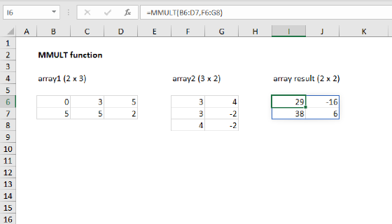
One option for solving this problem is the MMULT function. The MMULT function returns the matrix product of two arrays, sometimes called the "dot product". The result from MMULT is an array that contains the same number of rows as array1 and the same number of columns as array2. The MMULT function takes two arguments, array1 and array2, both of which are required. The column count of array1 must equal the row count of array2. In the example shown, the formula in G6 is:
=SUM(--(MMULT(--(data=G4),TRANSPOSE(COLUMN(data)^0))>0))
Working from the inside out, the logical criteria used in this formula is:
--(data=G4)
where data is the named range B4:D15. This expression generates a TRUE or FALSE result for every value in data, and the double negative (--) coerces the TRUE FALSE values to 1s and 0s, respectively. The result is an array of 1s and 0s like this:
{1,0,1;0,0,0;1,0,0;0,0,0;0,0,0;0,0,0;0,0,0;0,1,1;0,0,0;0,0,0;1,0,0;0,1,0}
Like the original data, this array is 12 rows by 3 columns (12 x 3) and is delivered directly to the MMULT function as array1. Array2 is derived with this snippet:
TRANSPOSE(COLUMN(data)^0)
Which returns an array of three 1s like this:
{1;1;1}
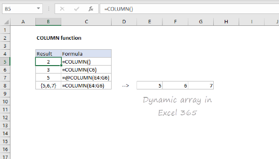
This is the tricky and fun part of this formula. The COLUMN function is used for convenience as a way to generate a numeric array of the right size. To perform matrix multiplication with MMULT, the column count in array1 (3) must equal the row count in array2 (3). COLUMN returns the 3-column array {2,3,4} which, when raised to the power of zero, becomes {1,1,1}. Next, the TRANSPOSE function transposes the 1 x 3 array into a 3 x 1 array:
TRANSPOSE({1,1,1}) // returns {1;1;1}
With both arrays in place, the MMULT function runs and returns an array with 12 rows and 1 column, {2;0;1;0;0;0;0;2;0;0;1;1}. This array contains the count per row of cells that contain 19, and we can use this data to solve the problem. Each non-zero number represents a row that contains the number 19, so we can convert non-zero values to 1s and sum up the result:
=SUM(--({2;0;1;0;0;0;0;2;0;0;1;1}>0))
We check for non-zero entries with >0 and again coerce TRUE FALSE to 1 and 0 with a double negative (--) to get a final array inside SUM:
=SUM({1;0;1;0;0;0;0;1;0;0;1;1})
In this array, 1 represents a row that contains 19 and a 0 represents a row that does not contain 19. The SUM function returns a final result of 5, the count of all rows that contain the number 19.
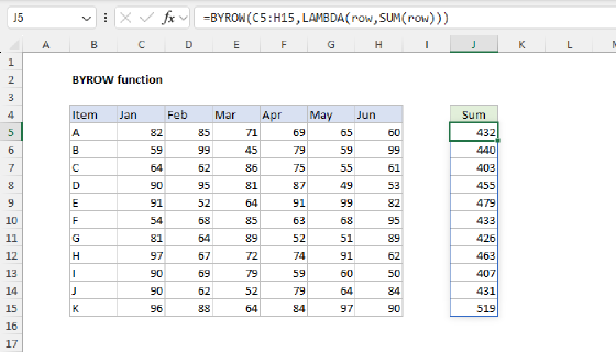
BYROW option
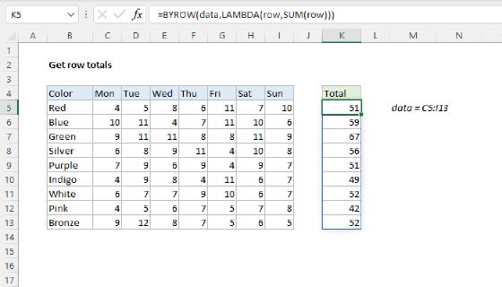
The BYROW function applies a LAMBDA function to each row in a given array and returns one result per row as a single array. The purpose of BYROW is to process data in an array or range in a "by row" fashion. For example, if BYROW is given an array with 12 rows, BYCOL will return an array with 12 results. In this example, we can use BYROW like this:
=SUM(BYROW(data,LAMBDA(row,--(SUM(--(row=G4))>0))))
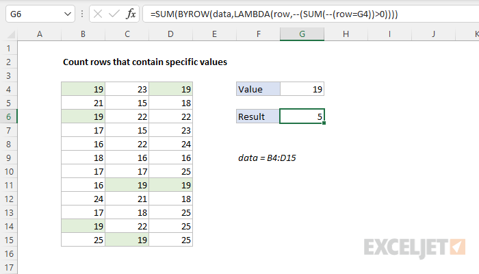
The BYROW function iterates through the named range data (B4:D15) one row at a time. At each row, BYCOL evaluates and stores the result of the supplied LAMBDA function:
LAMBDA(row,--(SUM(--(row=G4))>0))
The logic here checks for values in row that are equal to G4, which results in an array of TRUE and FALSE values. The TRUE and FALSE values are coerced to 1s and 0s with the double negative (--), and the SUM function sums the result. Next, we check if the total from SUM is >0, and coerce that result to a 1 or 0. After BYROW runs, we have an array with one result per row, either a 1 or 0:
{1;0;1;0;0;0;0;1;0;0;1;1} // result from BYROW
The formula can now be simplified as follows:
=SUM({1;0;1;0;0;0;0;1;0;0;1;1}) // returns 5
In the last step, the SUM function sums the items in the array and returns a final result of 5.
Literal contains
To check for specific substrings (i.e. check to see if cells contain a specific text value) you can adjust the logic in the formulas above to use the ISNUMBER and SEARCH functions. For example, to check if a value contains "apple" you can use:
=ISNUMBER(SEARCH("apple",data))
This expression would replace data=G4 logic above like this:
=SUM(--(MMULT(--(ISNUMBER(SEARCH(G4,data))),TRANSPOSE(COLUMN(data)^0))>0))
See this example for more information on using ISNUMBER with SEARCH.