Summary
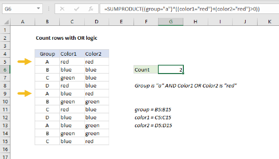
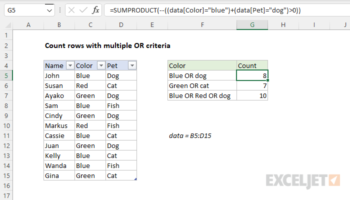
To count rows using multiple criteria in different columns with OR logic you can use the SUMPRODUCT function. In the example shown, the formula in G5 is:
=SUMPRODUCT(--((data[Color]="blue")+(data[Pet]="dog")>0))
where data is an Excel Table in the range B5:D15. The result is 8, the count of rows where Color is "Blue" OR Pet is "Dog".
Generic formula
=SUMPRODUCT(--((criteria1)+(criteria2)>0))
Explanation
In this example, the goal is to count rows using OR logic based on the criteria shown in column F. For example, in cell G5 we want to count rows where Color is "Blue" OR Pet is "Dog". This can be done with Boolean logic and the SUMPRODUCT function, as explained below.
Notes
- This formula uses an Excel Table named data to hold all data. As a result, the formula uses structured references to refer to columns in the table. The key benefit is that the table will automatically expand to include new data in the calculated results.
- Excel formulas are not case-sensitive by default, so we are using lowercase in all logical tests for simplicity.
- The SUMPRODUCT function is used below for compatibility with Legacy Excel. In the current version of Excel, you can use the SUM function instead. For more on this topic, see: Why SUMPRODUCT?
Basic count
In the example shown, we want to count rows where Color is "blue", OR Pet is "dog". To count rows where Color is "Blue", we can start off like this:
=SUMPRODUCT(--(data[Color]="blue"))
Inside the SUMPRODUCT function, we compare all values in data[Color] with "Blue". Since there are 11 rows in the table, the result is an array with 11 TRUE and FALSE results like this:
{TRUE;FALSE;FALSE;TRUE;FALSE;FALSE;TRUE;FALSE;TRUE;TRUE;FALSE}
We want to count all the TRUE values with SUMPRODUCT. However, the SUMPRODUCT function will ignore the logical values TRUE and FALSE by default, so we first need to convert these values to their numeric equivalents, 1 and 0. To do this, we use a double negative (--). The result is an array of 1s and 0s like this:
{1;0;0;1;0;0;1;0;1;1;0}
This array is returned directly to the SUMPRODUCT function:
=SUMPRODUCT({1;0;0;1;0;0;1;0;1;1;0}) // returns 5
With just one array to process, SUMPRODUCT sums the array and returns a final result of 5. We now have a count of all rows where Color is "Blue". The next step is to implement the OR logic we need to add rows where the Pet is "Dog".
Implementing OR logic
In the example shown, we want to count rows where Color is "Blue" OR Pet is "Dog". When using Boolean Algebra in Excel formulas, multiplication corresponds to AND logic and addition corresponds to OR logic. This means we want to use the addition operator (+) to extend our formula like this:
=(data[Color]="blue")+(data[Pet]="dog")
We are now performing two logical tests, one for each condition, joined with addition. Each expression in the formula above returns an array with 11 TRUE and FALSE results:
={TRUE;FALSE;FALSE;TRUE;FALSE;FALSE;TRUE;FALSE;TRUE;TRUE;FALSE}+{TRUE;FALSE;TRUE;FALSE;TRUE;FALSE;FALSE;TRUE;FALSE;FALSE;FALSE}
Next, the math operation of addition automatically converts the TRUE and FALSE values to 1s and 0s, and the result is a single numeric array like this:
{2;0;1;1;1;0;1;1;1;1;0}
We are making progress, but notice the array contains the number 2. This corresponds to the first row, where Color is "Blue" and Pet is "Dog". In other words, rows where both tests return TRUE will generate 2s in our calculation, which means we may double count some rows. To guard against this, we check if results are greater than 0 like this:
=(data[Color]="blue")+(data[Pet]="dog")>0
This expression returns 11 TRUE and FALSE results like this:
{TRUE;FALSE;TRUE;TRUE;TRUE;FALSE;TRUE;TRUE;TRUE;TRUE;FALSE}
This is close to what we need, but notice we have lost our numeric array in the process. This happened because checking if values are greater than zero converted the numbers back to TRUE and FALSE values. To get a numeric result, we again need a double negative (--):
--((data[Color]="blue")+(data[Pet]="dog")>0)
This returns the following numeric array, containing only 1s and 0s:
{1;0;1;1;1;0;1;1;1;1;0}
The 1s correspond to rows where Color is "Blue" OR Pet is "Dog" and the 0s correspond to rows where neither condition is true. Putting it all back together, the formula in G5 is solved like this:
=SUMPRODUCT(--((data[Color]="blue")+(data[Pet]="dog")>0))
=SUMPRODUCT(--({2;0;1;1;1;0;1;1;1;1;0}>0))
=SUMPRODUCT({1;0;1;1;1;0;1;1;1;1;0})
=8
Green OR Cat
The formula to count rows where Color is "Green" OR Pet is "Cat", we use exactly the same approach. The formula in G6 is:
=SUMPRODUCT(--((data[Color]="green")+(data[Pet]="cat")>0))
=SUMPRODUCT(--({0;1;1;0;1;0;1;1;1;0;2}>0))
=SUMPRODUCT({0;1;1;0;1;0;1;1;1;0;1}) // returns 7
The final count in this case is 7.
Blue OR Red OR dog
The formula in G7 extends the original formula to count Red or Blue:
=SUMPRODUCT(--((data[Color]="blue")+(data[Color]="red")+(data[Pet]="dog")>0))
=SUMPRODUCT(--({2;1;1;1;1;1;1;1;1;1;0}>0))
=SUMPRODUCT({1;1;1;1;1;1;1;1;1;1;0}) // returns 10
The final result is 10.
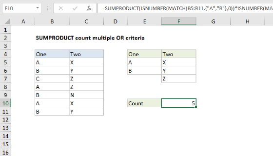
Many values with OR logic
If you need to test for many values, adding new logical tests becomes tedious. This example shows a more advanced approach.
Other logical tests
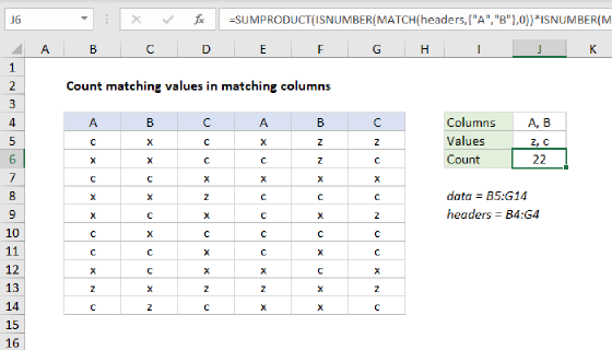
The example shown tests for simple equality, but you can replace those statements with other logical tests as needed. For example, to count rows where cells in column A contain "red" OR cells in column B contain "blue", you could use a formula like this:
=SUMPRODUCT(--(ISNUMBER(SEARCH("red",A1:A10))+ISNUMBER(SEARCH("blue",B1:B10))>0))
See more information about ISNUMBER with SEARCH here.
More conditions
To handle more conditions, just add more logical tests inside the SUMPRODUCT function, using parentheses to control the order of operations where necessary.