Summary
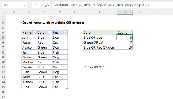
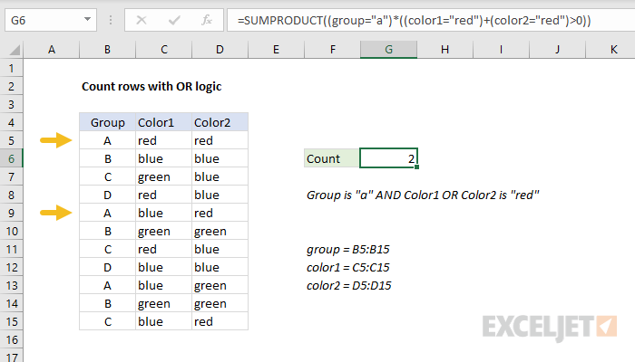
To count rows with OR logic, you can use a formula based on the SUMPRODUCT function. In the example shown, the formula in G6 is:
=SUMPRODUCT((group="a")*((color1="red")+(color2="red")>0))
where group (B5:B15), color1 (C5:C15), and color2 (D5:D15) are named ranges.
Explanation
One of the trickier problems in Excel is to count rows in a set of data with "OR logic". There are two basic scenarios: (1) you want to count rows where a value in a column is "x" OR "y" (2) you want to count rows where a value, "x", exists in one column OR another.
In this example, the goal is to count rows where group = "a" AND Color1 OR Color2 are "red". This means we are working with scenario 2 above.
With COUNTIFS
You might at first reach for the COUNTIFS function, which handles multiple criteria natively. However, the COUNTIFS function joins conditions with AND logic, so all criteria must be TRUE to be included in the count:
=COUNTIFS(group,"a",color1,"red",color2,"red") // returns 1
This makes COUNTIFS unworkable, unless we use multiple instances of COUNTIFS:
=COUNTIFS(group,"a",color1,"red")+COUNTIFS(group,"a",color2,"red")-COUNTIFS(group,"a",color1,"red",color2,"red")
Translation: count rows where group is "a" and color1 is "red" + count rows where group is "a" and color2 is "red". Then subtract the count of rows where group is "a" and color1 is "red" and color2 is "red" (to avoid double counting).
This works, but you can see this is a somewhat complicated and redundant formula.
With Boolean logic
A better solution is to use Boolean logic, and process the result with the SUMPRODUCT function. (If you need a primer on Boolean algebra, this video provides an introduction.) In the example shown, the formula in G6 is:
=SUMPRODUCT((group="a")*((color1="red")+(color2="red")>0))
where group (B5:B15), color1 (C5:C15), and color2 (D5:D15) are named ranges.
The first part of the problem is to test for group = "a" which we do like this:
(group="a")
Because the range B5:B15 contains 11 cells, this expression returns an array of 11 TRUE and FALSE values like this:
{TRUE;FALSE;FALSE;FALSE;TRUE;FALSE;FALSE;FALSE;TRUE;FALSE;FALSE}
Each TRUE represents a row where the group is "A".
Next, we need to check for the value "red" in either color1 or color2. We do this with two expressions joined by addition (+), since addition corresponds with OR logic in Boolean algebra:
(color1="red")+(color2="red")
Excel automatically evaluates TRUE and FALSE values as 1s and 0s during any math operation, so the result from the above expression is an array like this:
{2;0;0;1;1;0;1;0;0;0;1}
The first number in the array is 2, because both Color1 and Color2 are "red" in the first row. For reasons explained below, we need to guard against this situation by checking for values greater than zero:
({2;0;0;1;1;0;1;0;0;0;1})>0
Now we again have an array of TRUE and FALSE values:
{TRUE;FALSE;FALSE;TRUE;TRUE;FALSE;TRUE;FALSE;FALSE;FALSE;TRUE}
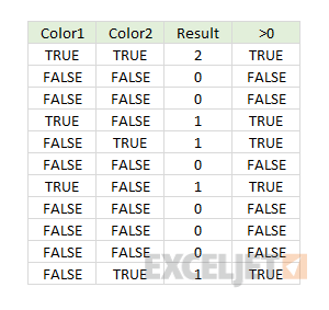
The table below summarizes how Excel evaluates the color logic explained above:
At this point, we have results from testing Group ="a" in one array:
{TRUE;FALSE;FALSE;FALSE;TRUE;FALSE;FALSE;FALSE;TRUE;FALSE;FALSE}
And results from testing "red" in Color1 or Color2 in another array:
{TRUE;FALSE;FALSE;TRUE;TRUE;FALSE;TRUE;FALSE;FALSE;FALSE;TRUE}
The next step is to bring these two arrays together with "AND logic". To do this, we use multiplication (*), since multiplication corresponds to AND logic in Boolean algebra.
After multiplying the two arrays together, we have a single array of 1s and 0s, which is delivered directly to the SUMPRODUCT function:
=SUMPRODUCT({1;0;0;0;1;0;0;0;0;0;0})
The SUMPRODUCT function returns the sum of numbers, 2, as a final result. This is the count of rows where group = "a" AND Color1 OR Color2 are "red".
To avoid double counting
We don't want to double count rows where both Color1 and Color2 are "red". This is why we check the results from (color1="red")+(color2="red") for values greater than zero in the code below:
((color1="red")+(color2="red"))>0
Without this check, the 2 from the first row in the data would show up in the final array, and cause the formula to incorrectly return 3 as the final count.
FILTER option
One nice thing about Boolean logic is that it works perfectly with Excel's newest functions, like XLOOKUP and FILTER. For example, the FILTER function can use exactly the same logic explained above to extract matching rows:
=FILTER(B5:D15,(group="a")*((color1="red")+(color2="red")>0))
The result from FILTER is the two rows that meet criteria, as seen below:

If you'd like to learn more about these new functions, we have an overview, and video training.