Summary
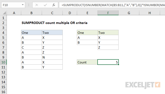
To count matching rows with multiple OR criteria, you can use a formula based on the SUMPRODUCT function. In the example shown, the formula in F10 is:
=SUMPRODUCT(ISNUMBER(MATCH(B5:B11,{"A","B"},0))*
ISNUMBER(MATCH(C5:C11,{"X","Y","Z"},0)))
This formula returns a count of rows where the value in column one is A or B and the value in column two is X, Y, or Z.
Generic formula
=SUMPRODUCT(ISNUMBER(MATCH(rng1,{"A","B"},0))*ISNUMBER(MATCH(rng2,{"X","Y","Z"},0)))
Explanation
In this example, the goal is to count rows where the value in column one is "A" or "B" and the value in column two is "X", "Y", or "Z". In the worksheet shown, we are using array constants to hold the values of interest, but the article also shows how to use cell references instead. In simple scenarios, you can use Boolean logic and the addition operator (+) to count with OR logic, but as the number of values being testing increases, the formula becomes unwieldy. To keep the formula as tidy as possible, this example uses the MATCH function together with the ISNUMBER function to check more than one value at a time.
ISNUMBER + MATCH
Working from the inside out, each condition is applied with a separate ISNUMBER + MATCH expression. To generate a count of rows in column one where the value is A or B we use the following code:
ISNUMBER(MATCH(B5:B11,{"A","B"},0)
Notice the values "A" and "B" are supplied as an array constant and match_type is set to zero for an exact match.
Note: the configuration for MATCH may appear "reversed" from what you might expect. This is necessary in order to preserve the structure of the source data in the results returned by MATCH, i.e. we get back seven results, one for each row in B5:B11.
Since we give the MATCH function 7 values to look for, MATCH returns an array that contains 7 results like this:
{1;2;#N/A;1;2;1;2}
Each number in this array represents a match on "A" or "B" in Column B (1="A", 2="B"). An #N/A error indicates a row where neither value was found. These results are delivered directly to the ISNUMBER function, which is used to convert the values from MATCH into simple TRUE and FALSE results:
ISNUMBER({1;2;#N/A;1;2;1;2})
ISNUMBER returns a new array that looks like this:
{TRUE;TRUE;FALSE;TRUE;TRUE;TRUE;TRUE}
In this array, TRUE values represent rows where "A" or "B" were found in column B. The next step is to test for "X","Y",or "Z" in column C, and for this we use exactly the same approach:
ISNUMBER(MATCH(C5:C11,{"X","Y","Z"},0))
With the above configuration, the MATCH function returns the following array:
{1;2;3;3;#N/A;1;2}
As before, the ISNUMBER function converts these results to TRUE and FALSE values and returns an array like this:
{TRUE;TRUE;TRUE;TRUE;FALSE;TRUE;TRUE}
We now have everything we need to perform the count, and for this we use the SUMPRODUCT function.
SUMPRODUCT function
The final step in the formula is to tally up the rows that meet the criteria outlined above. In the example shown, the formula in F10 is:
=SUMPRODUCT(ISNUMBER(MATCH(B5:B11,{"A","B"},0))*
ISNUMBER(MATCH(C5:C11,{"X","Y","Z"},0)))
After the two MATCH and ISNUMBER expressions are evaluated, the formula simplifies to the following:
=SUMPRODUCT({TRUE;TRUE;FALSE;TRUE;TRUE;TRUE;TRUE}*{TRUE;TRUE;TRUE;TRUE;FALSE;TRUE;TRUE})
Next, the two arrays are multiplied together inside SUMPRODUCT, which automatically converts TRUE FALSE values to 1s and 0s as a result of the math operation:
=SUMPRODUCT({1;1;0;1;1;1;1}*{1;1;1;1;0;1;1})
Once the two arrays are multiplied together, we have a single array like this:
=SUMPRODUCT({1;1;0;1;0;1;1}) // returns 5
In this array, a 1 signifies a row that meets all criteria and a 0 indicates a row that does not. With just a single array to process, SUMPRODUCT sums the array and returns a final result of 5.
With cell references
The example above uses hardcoded array constants, but you can also use cell references:
=SUMPRODUCT(ISNUMBER(MATCH(B5:B11,E5:E6,0))*ISNUMBER(MATCH(C5:C11,F5:F7,0)))
This approach can be "scaled up" to handle more criteria. You can see an example in this formula challenge.
Note: The SUMPRODUCT function is used below for compatibility with Legacy Excel. In the current version of Excel, you can use the SUM function instead. For more on this topic, see: Why SUMPRODUCT?