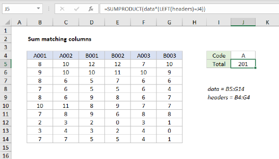
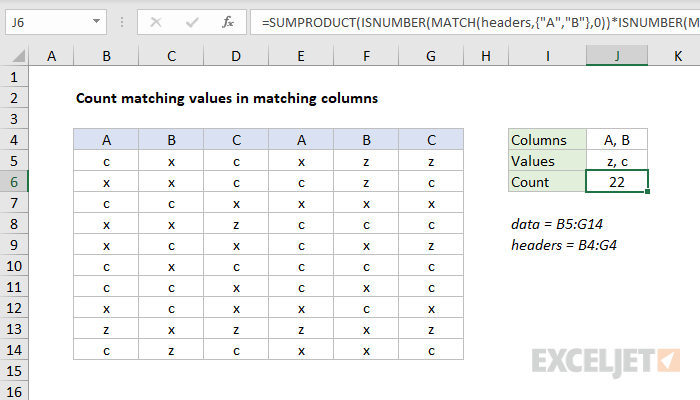
Count matching values in matching columns

In this example, the goal is to count "z" or "c" values in the named range data, but only when the column header is "A" or "B". The formula used to perform this calculation is based on the SUMPRODUCT function:

=SUMPRODUCT(ISNUMBER(MATCH(headers,{"A","B"},0))*ISNUMBER(MATCH(data,{"z","c"},0)))

Working from the inside out, note that SUMPRODUCT contains a single argument, which is composed of this expression:

ISNUMBER(MATCH(headers,{"A","B"},0))*ISNUMBER(MATCH(data,{"z","c"},0))

This expression is formed from two parts, each representing a logical test. The left part tests column headers, and the right tests values.  The two parts are joined with multiplication (*) because the overall logic is AND, and multiplication corresponds to AND in Boolean algebra.

On the left, the MATCH function is used with the ISNUMBER function to match target columns:

ISNUMBER(MATCH(headers,{"A","B"},0)) // match "A" or "B"

Inside MATCH, notice the arguments are "reversed" to maintain the existing data structure: the header values are used for the lookup_value argument, and the array argument is provided as an array constant that contains the values we are looking for, "A" and "B". The result from MATCH is an array composed of #N/A errors or numbers. The numbers indicate matched positions:

{1,2,#N/A,1,2,#N/A}

There are 6 items in this array because we are testing 6 columns. The numbers represent matched columns and errors represent columns that do not match. This array is returned and handed off to the ISNUMBER function:

ISNUMBER({1,2,#N/A,1,2,#N/A}) // convert to TRUE or FALSE

which returns an array like this:

{TRUE,TRUE,FALSE,TRUE,TRUE,FALSE}

Note the TRUE values correspond to columns that are either "A" or "B". This completes the column matching logic.

On the right side of the expression, we have similar logic to test the values themselves:

ISNUMBER(MATCH(data,{"z","c"},0))

The MATCH function is again used to check for two values "z" or "c" with the same reversed argument approach. Because the named range data contains 60 values, the result from MATCH is an array with 60 values:

{2,#N/A,2,#N/A,1,1;#N/A,#N/A,2,2,1,2;2,2,#N/A,#N/A,#N/A,#N/A;#N/A,#N/A,1,2,2,2;#N/A,2,#N/A,2,#N/A,1;2,#N/A,2,2,2,2;2,2,#N/A,2,#N/A,2;#N/A,2,#N/A,#N/A,2,#N/A;1,#N/A,1,1,#N/A,1;2,1,2,#N/A,#N/A,2}

The ISNUMBER function again translates this array into TRUE and FALSE values:

{TRUE,FALSE,TRUE,FALSE,TRUE,TRUE;FALSE,FALSE,TRUE,TRUE,TRUE,TRUE;TRUE,TRUE,FALSE,FALSE,FALSE,FALSE;FALSE,FALSE,TRUE,TRUE,TRUE,TRUE;FALSE,TRUE,FALSE,TRUE,FALSE,TRUE;TRUE,FALSE,TRUE,TRUE,TRUE,TRUE;TRUE,TRUE,FALSE,TRUE,FALSE,TRUE;FALSE,TRUE,FALSE,FALSE,TRUE,FALSE;TRUE,FALSE,TRUE,TRUE,FALSE,TRUE;TRUE,TRUE,TRUE,FALSE,FALSE,TRUE}

Now the original expression above (inside SUMPRODUCT) can be written like this:

{TRUE,TRUE,FALSE,TRUE,TRUE,FALSE}*{TRUE,FALSE,TRUE,FALSE,TRUE,TRUE;FALSE,FALSE,TRUE,TRUE,TRUE,TRUE;TRUE,TRUE,FALSE,FALSE,FALSE,FALSE;FALSE,FALSE,TRUE,TRUE,TRUE,TRUE;FALSE,TRUE,FALSE,TRUE,FALSE,TRUE;TRUE,FALSE,TRUE,TRUE,TRUE,TRUE;TRUE,TRUE,FALSE,TRUE,FALSE,TRUE;FALSE,TRUE,FALSE,FALSE,TRUE,FALSE;TRUE,FALSE,TRUE,TRUE,FALSE,TRUE;TRUE,TRUE,TRUE,FALSE,FALSE,TRUE}

Note the multiplication operator is still there, just after the first array. In Excel any math operation will automatically convert TRUE and FALSE values to their numeric equivalents, 1 and 0. This means you can think of the expression like this:

{1,1,0,1,1,0}*{1,0,1,0,1,1;0,0,1,1,1,1;1,1,0,0,0,0;0,0,1,1,1,1;0,1,0,1,0,1;1,0,1,1,1,1;1,1,0,1,0,1;0,1,0,0,1,0;1,0,1,1,0,1;1,1,1,0,0,1}

After the expression is evaluated, we have a single array like this:

{1,0,0,0,1,0;0,0,0,1,1,0;1,1,0,0,0,0;0,0,0,1,1,0;0,1,0,1,0,0;1,0,0,1,1,0;1,1,0,1,0,0;0,1,0,0,1,0;1,0,0,1,0,0;1,1,0,0,0,0}

This array is delivered to the SUMPRODUCT function as the array1 argument. Then, with only one array to process, SUMPRODUCT sums the items in the array and returns a final result: 22.

Note: although SUMPRODUCT can handle multiple arrays as separate arguments, you will see many formulas that place all logic into a single argument. Doing so takes advantage of the fact that Excel automatically coerces TRUE and FALSE values to 1s and 0s during any math operation. When the logic is separated into separate arrays, an additional step must be taken to convert to 1s and 0s. For more details, see Why SUMPRODUCT?

Contains logic

In the example shown above testing logic is "equal to". The columns must be equal to "A" or "B" and the values must be equal to "z" or "c". But sometimes you need to test with "contains" logic. For example, test for values that contain "z" or contain "c".

One consequence of reversing the arguments inside the MATCH function is that wildcards can't be used with the lookup values, because these values appear as the array argument. If you need to test values using contains logic, you can switch to another approach based on ISNUMBER with the SEARCH function. For example, to match values that contain "x" or "c", you can use an expression like this:

=ISNUMBER(SEARCH("z",data))+ISNUMBER(SEARCH("c",data))

Note we are joining each test with the addition operator (+) because in Boolean algebra addition corresponds to OR logic. The final formula would then look like this:

=SUMPRODUCT(ISNUMBER(MATCH(headers,{"A","B"},0))*(ISNUMBER(SEARCH("z",data))+ISNUMBER(SEARCH("c",data))))

Note an additional set of parentheses () have been added to control order of operations.