Sum every nth column

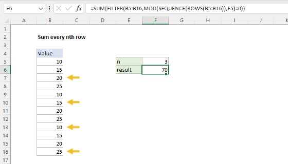
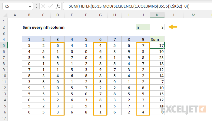
To sum every nth column (i.e. every second column, every third column, etc.) you can use a formula based on the FILTER function, the MOD function, and the SUM function. In the example shown, the formula in cell K5, copied down, is:

=SUM(FILTER(B5:J5,MOD(SEQUENCE(1,COLUMNS(B5:J5)),$K$2)=0))

With the number 3 in cell K2 for n, the result is 17. As the formula is copied down, we get a new sum on each row. Each result is the sum of every third value from column B to column J.

Note: With a small set of data, you can easily enter a formula manually to sum columns as you like. The point of this example is to show how to create a general solution that will scale up to a larger set of data, and allow the value for n to be easily changed.

Explanation

In this example, the goal is to sum every nth value by column in a range of data, as seen in the worksheet above. For example, if n=2, we want to sum every second value by column, if n=3, we want to sum every third value by column, and so on. All data is in the range B5:J16 and n is entered into cell K2 as 3. The value for n can be changed at any time. There are two basic approaches to this problem in Excel:

Extract nth column values & sum the result
Zero-out non-nth values & sum the result

In the current version of Excel, a good way to solve the problem is with approach #1 and the FILTER function. In Legacy Excel, you can use approach #2 and a formula based on the SUMPRODUCT function. Both approaches are explained below.

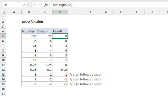
Note: The approaches below all depend on the MOD function to work out which values to sum. The MOD function returns the remainder of two numbers after division, and you will often see it in formulas that deal with repeating values.

Example formula

In the example shown, the formula in cell K5 is:

=SUM(FILTER(B5:J5,MOD(SEQUENCE(1,COLUMNS(B5:J5)),$K$2)=0))

At a high level, this formula uses the FILTER function to extract values associated with every nth column of the data, and the SUM function to sum the values extracted.

Extracting data

Working from the inside out, the first step in this problem is to collect the data that should be summed. This is done with the FILTER function like this:

FILTER(B5:J5,include)

where include represents the formula logic needed to target every nth value by column (every 3rd value in the example). To construct the logic we need, we use a combination of the MOD function, the SEQUENCE function, and the COLUMNS function:

MOD(SEQUENCE(1,COLUMNS(B5:J5)),$K$2)=0

The COLUMNS function returns the count of columns in the range B5:J5, which is 9:

MOD(SEQUENCE(1,9),$K$2)=0

With 1 as the rows argument and 9 as the columns argument, the SEQUENCE function returns a numeric array of 9 numbers like this:

{1,2,3,4,5,6,7,8,9}

Notice the commas in this array indicate that this is a horizontal array, 1 row x 9 columns. Substituting the array above and the value for n (3) into the formula we have:

MOD({1,2,3,4,5,6,7,8,9},3)=0

The MOD function returns the remainder of each number in the array divided by 3:

{1,2,0,1,2,0,1,2,0}=0

The result from MOD is compared to zero, which creates an array of TRUE and FALSE values:

{FALSE,FALSE,TRUE,FALSE,FALSE,TRUE,FALSE,FALSE,TRUE}

Note that every third value is TRUE. These are the values we want to sum.

The array above is returned to FILTER as the include argument. FILTER uses this array to "filter" values in the range B5:J16 by column. Only values associated with TRUE make it through the filter operation. The result is an array that contains every 3rd value in the data. Since there are 9 values total, FILTER returns 3 values directly to the SUM function:

=SUM({6,4,7}) // returns 17

The SUM function sums the array and returns 17 as a final result. This formula is dynamic. For example, if the value for n in cell K2 is changed to 2 (every 2nd value) the new result is 16.

Legacy Excel formula

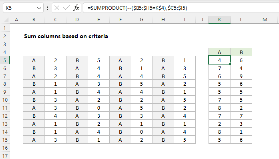
In older versions of Excel that do not include the FILTER or SEQUENCE functions, you can use a different formula based on the SUMPRODUCT function:

=SUMPRODUCT(--(MOD(COLUMN(B5:J5)-COLUMN(B5)+1,$K$2)=0),B5:J5)

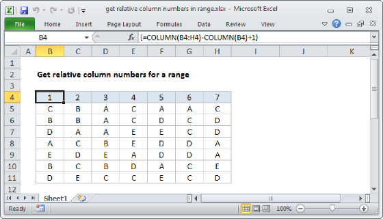
The concept is similar to the formula explained above but the approach is different. Rather than extracting values of interest from the data, this formula "zeros out" values not of interest. First, the formula uses the COLUMN function to construct a relative set of column numbers:

COLUMN(B5:J5)-COLUMN(B5)+1

The result is a numeric array like this:

{1,2,3,4,5,6,7,8,9}

As above, is a horizontal array, 1 row x 9 columns. Inside the SUMPRODUCT function, we again use the MOD function to construct a filter:

MOD(COLUMN(B5:J5)-COLUMN(B5)+1,$K$2)=0
MOD({1,2,3,4,5,6,7,8,9},3)=0)

MOD returns an array of TRUE FALSE values like this:

{FALSE,FALSE,TRUE,FALSE,FALSE,TRUE,FALSE,FALSE,TRUE}

Note that every 3rd value is TRUE. A double negative (--) is used to convert the TRUE and FALSE values to 1s and 0s. Back in the SUMPRODUCT, we now have:

=SUMPRODUCT({0,0,1,0,0,1,0,0,1},B5:J5)

The SUMPRODUCT then multiplies the two arrays together and returns the sum of products. Only the values in B5:J5 that are associated with 1s survive this operation, the other values are "zeroed out":

=SUMPRODUCT({0,0,6,0,0,4,0,0,7}) // returns 17

The final result is 17. This formula is also dynamic. If the value for n in cell K2 is changed to 2 (every 2nd value) the new result is 16.

Hybrid approach

Yet another approach is to create a more modern version of the SUMPRODUCT formula above by replacing SUMPRODUCT with SUM, and the COLUMN construction with SEQUENCE:

=SUM((MOD(SEQUENCE(1,COLUMNS(B5:J5)),$K$2)=0)*B5:J5)

This formula works the same way as the SUMPRODUCT formula above, but the SEQUENCE function is a simpler way to generate a relative set of column numbers. Notice that because we have replaced SUMPRODUCT with SUM, we need to move all logic into the first argument and do our own multiplication. This formula will only work in the current version of Excel.