Sum every nth row

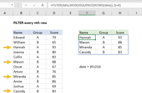
In this example, the goal is to sum every nth value in a range of data, as seen in the worksheet above. For example, if n=2, we want to sum every second value (every other value), if n=3, we want to sum every third value, and so on. All data is in the range B5:B16 and n is entered into cell F5 as 3. This value can be changed at any time. In the latest version of Excel, the easiest way to do this is to use the FILTER function. In Legacy Excel, you can use an alternative formula based on the SUMPRODUCT function as explained below.

Example formula

In the example shown, the formula in cell F6 is:

=SUM(FILTER(B5:B16,MOD(SEQUENCE(ROWS(B5:B16)),F5)=0))

At a high level, this formula uses the FILTER function to extract values associated with every nth row of the data, and the SUM function to sum the values extracted.

Extracting data

Working from the inside out, the first step in this problem is to collect the data that should be summed. This is done with the FILTER function like this:

FILTER(B5:B16,include)

where include represents the formula logic needed to target every nth value (every 3rd value in the example). To construct the logic we need, we use a combination of the MOD function, the SEQUENCE function, and the ROWS function:

MOD(SEQUENCE(ROWS(B5:B16)),F5)=0)

The ROWS function returns the count of rows in the range B5:B16, which is 12:

MOD(SEQUENCE(12),F5)=0)

With 12 as the rows argument, the SEQUENCE function returns a numeric array of 12 numbers like this:

{1;2;3;4;5;6;7;8;9;10;11;12}

Substituting the array above and the value for n (3) into the formula we have:

MOD({1;2;3;4;5;6;7;8;9;10;11;12},3)=0)

The MOD function returns the remainder of each number in the array divided by 3:

{1;2;0;1;2;0;1;2;0;1;2;0}=0

The result from MOD is compared to zero, which creates an array of TRUE and FALSE values:

{FALSE;FALSE;TRUE;FALSE;FALSE;TRUE;FALSE;FALSE;TRUE;FALSE;FALSE;TRUE}

Note that every third value is TRUE. This is the value returned to FILTER as the include argument. FILTER uses this array to "filter" values in the range B5:B16. Only values associated with TRUE make it through the filter operation. The result is an array that contains every 3rd value in the data. Since there are 12 values total, FILTER returns 4 values:

{20;15;10;25}

FILTER delivers this array of values directly to the SUM function, which returns the sum (70) as a final result:

SUM ({20;15;10;25}) // returns 70

This formula is dynamic. For example, if the value for n in cell F5 is changed to 2 (every 2nd value) the new result is 120.

Legacy Excel formula

In older versions of Excel that do not include the FILTER or SEQUENCE functions, you can use a different formula based on the SUMPRODUCT function:

=SUMPRODUCT(--(MOD(ROW(B5:B16)-ROW(B5)+1,F5)=0),B5:B16)

The concept is similar to the formula explained above but the approach is different. Rather than extract values of interest from the data, this formula "zeros out" the other values not of interest. First, the formula uses the ROW function to construct a relative set of row numbers:

ROW(B5:B16)-ROW(B5)+1

The result is a numeric array like this:

{1;2;3;4;5;6;7;8;9;10;11;12}

Inside the SUMPRODUCT function, we again use the MOD function to construct a filter:

=MOD(ROW(B5:B16)-ROW(B5)+1,F5)=0
=MOD({1;2;3;4;5;6;7;8;9;10;11;12},F5)=0

MOD returns an array of TRUE FALSE values like this:

{FALSE;FALSE;TRUE;FALSE;FALSE;TRUE;FALSE;FALSE;TRUE;FALSE;FALSE;TRUE}

Again, note that every 3rd value is TRUE. A double negative (--) is used to convert the TRUE and FALSE values to 1s and 0s. Back in the SUMPRODUCT, we now have:

=SUMPRODUCT({0;1;0;1;0;1;0;1;0;1;0;1},B5:B16)

The SUMPRODUCT then multiplies the two arrays together and returns the sum of products. Only the values in B5:B6 that are associated with 1s survive this operation, the other values are "zeroed out":

=SUMPRODUCT({0;0;20;0;0;15;0;0;10;0;0;25}) // returns 70

The final result is 70. This formula is also dynamic. If the value for n in cell F5 is changed to 2 (every 2nd value) the new result is 120.