Summary
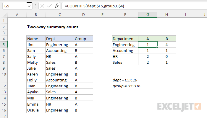
To build a two-way summary count, you can use the COUNTIFS function. In the example shown, the formula in G5 is:
=COUNTIFS(dept,$F5,group,G$4)
where dept (B5:B16) and group (C5:C16) are named ranges. The explanation below also includes a solution where source data is in an Excel Table.
Generic formula
=COUNTIFS(range1,criteria1,range2,criteria2)
Explanation
In this example, the goal is to count the people shown in the table by both Department (Dept) and Group as shown in the worksheet. A simple way to do this is with the COUNTIFS function.
COUNTIFS function
The COUNTIFS function is designed to count things based on more than one condition. Conditions are supplied to COUNTIFS in range/criteria "pairs" like this:
=COUNTIFS(range1,criteria1,range2,criteria2)
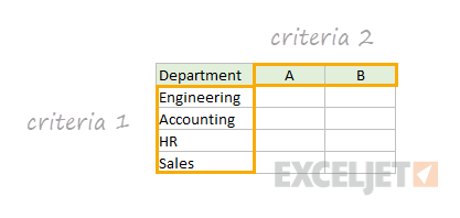
In this problem, the first step is to create the shell of the summary table that contains one set of criteria in the left-most column, and the second set of criteria in the top row as column headers like this:
The next step is to enter the COUNTIFS function in cell G5 with the first condition for Department:
=COUNTIFS(dept,$F5
For criteria_range1, we use the named range dept (B5:B16). For criteria1, we use the mixed reference $F5. Cell F5 contains the value "Engineering", which will be used for criteria. We use a mixed reference to lock the column only so that the formula will still refer to column F when we copy it to the next column. We leave the row relative because we want the row to change as we copy the formula down. Note that a named range automatically behaves like an absolute reference, so we don't need to do anything special with the range; it will not change when copied.
Next, we enter the second range/criteria pair to target values for Group:
=COUNTIFS(dept,$F5,group,G$4)
For criteria_range2, we use the named range group (C5:C16). For criteria2, we use the mixed reference G$4. Cell G4 contains the value "A", which will be used for criteria. We use a mixed reference to lock the row only so that the formula will still refer to row 4 when we copy it down.
This is the final formula entered in cell G5, and copied into the range G5:H8. To recap, the named ranges dept and group automatically behave like absolute references and will not change. The references to $F5 and G$4 however are mixed. As the formula is copied, the row in $F5 changes and the column in G$4 changes, which allows the COUNTIFS function to generate correct counts for all combinations of Department and Group.
Excel Table option
When you use an Excel Table to hold source data, you get some nice benefits, including a table that automatically expands when rows are added. Excel Tables use structured references, which appear automatically in formulas that refer to them. In the screen below, the formula in G5 is:
=COUNTIFS(data[[Dept]:[Dept]],$F5,data[[Group]:[Group]],G$4)
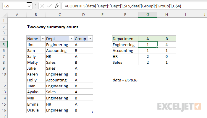
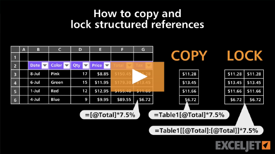
This formula is a bit more complex than usual, because the Dept and Group columns need to be locked in a special way with the double square brackets and a colon to allow the formula to be copied across the summary tabled. The two references below show this difference in syntax:
data[Dept] // normal
data[[Dept]:[Dept]] // locked
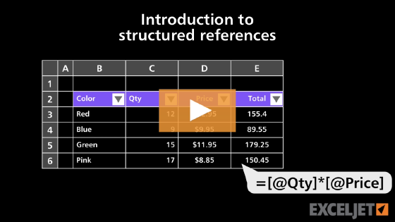
For more on Excel Tables and structured references, see the videos below. One of the videos shows an easy way to lock a structured reference. If you are new to Excel Tables, see What is an Excel Table?
Dynamic array option
In the latest version of Excel, which supports dynamic array formulas, you can adapt this example to automatically extract the values for Dept and Group with the UNIQUE function. If fact, if we throw in the LET function and two new functions, HSTACK and VSTACK, it is possible to write a single all-in-one formula that builds a complete summary table like this:
=LET(
  depts,UNIQUE(data[Dept]),
  groups,TRANSPOSE(UNIQUE(data[Group])),
  counts,COUNTIFS(data[Dept],depts,data[Group],groups),
  HSTACK(VSTACK({"Department"},depts),VSTACK(groups,counts))
)
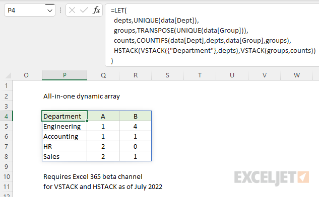
Note: VSTACK and HSTACK are still in beta, available via the Beta Channel for Excel 365.
In a nutshell, we use the UNIQUE function to extract unique departments and groups, and the COUNTIFS function to generate all counts. The LET function is used to assign all three intermediate results to the variables depts, groups, and counts. Next, the HSTACK and VSTACK functions are used to assemble the final table. Because HSTACK is the last function to run, it returns the final result, which is an array of values that spill into multiple cells. To learn more about how to convert a formula to use LET, see this detailed LET function example.
The best thing about this approach is that any changes to the source data will be reflected in the summary table instantly, with no need to refresh or edit the formula. As a bonus, there is no need to lock specific cell references. The formula above is a great example of how dynamic array formulas will completely change formula solutions in the future. See this example for another related problem with a more complete walkthrough.