Summary
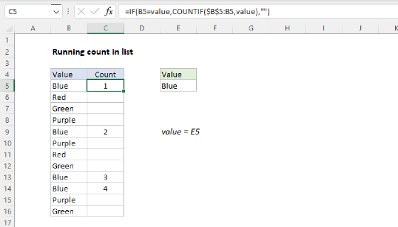
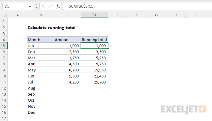
To calculate a running total (sometimes called a "cumulative sum") you can use the SUM function with an expanding reference. In the example shown, the formula in cell D5 is:
=SUM($C$5:C5)
As this formula is copied down the column, it calculates a running total on each row — a cumulative sum of all amounts up to that point.
Generic formula
=SUM($A$1:A1)
Explanation
In this example, the goal is to calculate a running total in column D of the worksheet as shown. A running total, or cumulative sum, is a set of partial sums that changes as more data is collected. Each calculation represents the sum of values up to that point. In this example, each calculation takes into account another month of the year. There are several ways to approach this problem, as explained below.
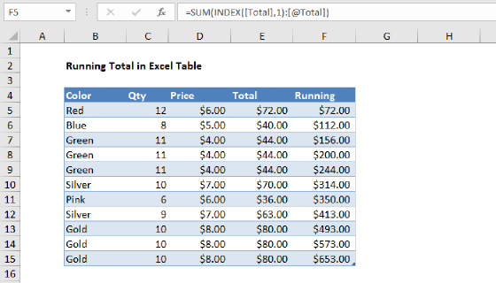
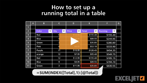
Note: if you want to create a running total in an Excel Table, you'll want to take a different approach from the formulas below. See this example.
SUM with expanding range
An easy way to create a running total in Excel is to use the SUM function with what is called an "expanding reference" — a special kind of reference that includes both absolute and relative parts. In the example shown, the formula in D5 is:
=SUM($C$5:C5)
Notice this range refers to one cell only (C5:C5). However, while the first reference to C5 on the left side of the colon (:) is an absolute reference ($C$5), the second reference is a relative reference (C5). As a result, when the formula is copied down the column, the left side of the range is "locked" and won't change, but the right side of the range is relative and will change at each new row. The result is that the range expands by one row each time it is copied down:
=SUM($C$5:C5) // formula in D5
=SUM($C$5:C6) // formula in D6
=SUM($C$5:C7) // formula in D7
=SUM($C$5:C8) // formula in D8
At each new row, the SUM function receives a larger range that includes the amount in the current row. The result is a cumulative sum of the values in column C up to that point.
Note: formulas with expanding ranges can cause performance problems in large sets of data. The formula below is more efficient.
SUM with two values
Another nice way to solve this problem is to use the SUM function to add the current amount to the previous cumulative sum. In cell D5, you can write a formula like this:
=SUM(C5,D4)
You can see this option in the screen below:
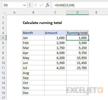
This may seem unusual, since D4 contains text, and not a number. However, the purpose of constructing the formula this way is to allow the same formula to be copied down the column without changes. Using the same formula in a column is considered a best practice because it makes things more consistent and reduces the chance of errors when formulas are copied. The reason we use the SUM function in this formula, instead of simple addition, is that SUM will automatically ignore text values. If we try instead to write a formula like this:
=C5+D4 // returns #VALUE!
The result is a #VALUE! error, because Excel's formula engine by default will not allow a number and text to be added together.
SCAN function
This problem can also be solved with the SCAN function, a new function in Excel designed to work with dynamic arrays. SCAN can be used to generate running totals and other calculations that show intermediate or incremental results. The SCAN function uses the LAMBDA function to apply the logic needed. The LAMBDA is applied to each value, and the result from SCAN is an array of results with the same dimensions as the original array. The structure of the LAMBDA used inside SCAN looks like this:
LAMBDA(a,v,calculation)
The first argument, a, is the accumulator used to create intermediate values. The accumulator begins as the initial_value provided to SCAN and changes as the SCAN function loops over the elements in array and applies a calculation. The v argument represents the value of each element in array. Calculation is the formula that creates the intermediate values that will appear in the final result. In this example, the basic SCAN formula to create a running total looks like this:
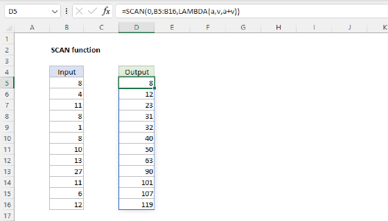
=SCAN(0,C5:C16,LAMBDA(a,v,a+v))
Notice the initial value of the accumulator is zero. At each new row, we simply add the current value (v) to the accumulator (a). Because we give SCAN an array that contains 12 values, SCAN will return an array with 12 results like this:
{1000;3500;5250;9750;15950;21450;25700;25700;25700;25700;25700;25700}
All twelve values will spill into the range D5:D16. To skip rows where the value in column C is not yet available, we can adapt the formula as follows:
=SCAN(0,C5:C16,LAMBDA(a,v,IF(v<>"",a+v,"")))
In this version, we check to see if the current value (v) is not empty. If so, we return a+v. If v is empty, we return an empty string (""). The array returned by SCAN with the modified LAMBDA looks like this:
{1000;3500;5250;9750;15950;21450;25700;"";"";"";"";""}
Here is the result on the worksheet:
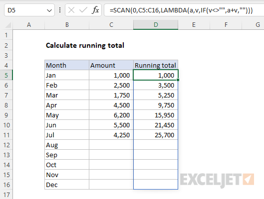
Notice the last five values are empty strings, which will display as blank cells in Excel. The key advantage to use SCAN in a problem like this is that it returns all results at the same time in a dynamic array. This makes it possible to use SCAN in more powerful all-in-one formulas.
Pivot Table
A Pivot Table is another good way to calculate running totals. See a basic example here.