Running count of occurrence in list

In this example, the goal is to create a running count for a specific value that appears in column B. The value to count is entered in cell E5, which is the named range value. The core of the solution explained below is the COUNTIF function, with help from the IF function to suppress a count for other values.

Basic count

Normally, the COUNTIF function is given a range and criteria like this:

COUNTIF(B5:B16,"blue") // returns 4

Since the range B5:B16 contains 4 cells that contain "blue", COUNTIF returns 4. The formula above works well when you want to single count for one value in a range. However, to get a running count, we'll need to adapt the formula to use an expanding range.

Running count with expanding range

An expanding range is a range with one side that is absolute, and one side that is relative. In this case, we lock the first reference to B5, and leave the second reference relative like this:

$B$5:B5 // expanding range

Notice that the left side of the range is locked ($B$5) and the right side is relative (B5). This is a special kind of "mixed reference", since it contains both absolute and relative addresses. Because the first reference, $B$5, is locked, it doesn't change. However the second reference, B5, changes when the formula is copied. The result is an expanding range. Dropping the expanding range back into the COUNTIF function, we have this formula:

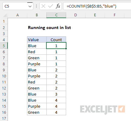
=COUNTIF($B$5:B5,"blue") // returns 1

As the formula is copied down column 1, the range "expands" at each row. You can see the result of the formula above in the screen below:

Notice we get a count on every row. However, the count only increments when another "blue" value is encountered.

Removing extra counts

Because we only want to create a running count for one specific value, the next step is to remove the counts that appear next to other values. To do this, we nest the COUNTIF function inside the IF function like this:

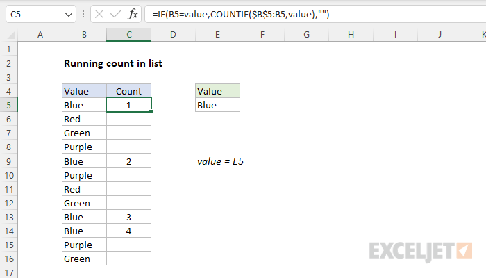
=IF(B5=value,COUNTIF($B$5:B5,value),"")

This is the formula entered in cell C5 of the example shown. Notice we have now swapped the hardcoded value "blue" with the named range value (E5). The named range is simply for convenience. It automatically acts like an absolute reference, and it makes the formula easier to read and write.

At each row, the logical test inside of IF tests the value in column B to see if it is equal to the named range value (E5), which contains "blue". If so, the COUNTIF formula explained above is executed, and returns the current running count for "blue". If the value in column B is not equal to "blue", the IF function returns an empty string (""). This effectively removes the count for all other values. The final result is a running count for cells that contain "blue".

Other values

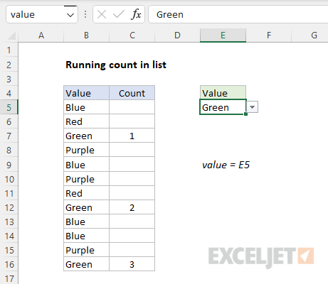
In the attached worksheet, the named range value (E5) is set up to provide a dropdown menu with data validation. If we select a different value, the running count formula immediately returns a new set of running counts. The screen below shows the result of selecting "Green" in E5:

SCAN solution

The SCAN function is designed for problems like running totals and running sums. However, it is not obvious how to use SCAN in this case because it isn't clear how to suppress the running count on non-matching rows. If we set the accumulator to an empty string (""), SCAN will return errors when we increment the accumulator on matching rows. One interesting solution is to run a logical test first, then feed the result into SCAN like this:

=LET(
hits,B5:B16=value,
counts,SCAN(0,hits,LAMBDA(a,v,a+v)),
IF(hits,counts,"")
)

In this formula, we use the LET function to define a variable called "hits" which is assigned a value based on the following expression:

B5:B16=value

With value equal to "Blue", this expression generates an array of 12 TRUE and FALSE values like this:

{TRUE;FALSE;FALSE;FALSE;TRUE;FALSE;FALSE;FALSE;TRUE;TRUE;FALSE;FALSE}

We then define another variable called "counts", and assign a value by scanning hits like this:

SCAN(0,hits,LAMBDA(a,v,a+v))

The result is that SCAN generates a running count using the TRUE values in hits. The math operation of a+v causes Excel to convert the TRUE value to 1, which increments a by 1. FALSE values evaluate as zero and do not affect the count. The resulting array looks like this:

{1;1;1;1;2;2;2;2;3;4;4;4}

The last step is to run counts through the IF function like this:

IF(hits,counts,"")

Here, the IF function acts like a filter. The numbers in counts associated with TRUE in hits pass through unaffected. The numbers associated with FALSE are replaced with empty strings. The array returned by IF looks like this:

{1;"";"";"";2;"";"";"";3;4;"";""}

The final result is the same as with the original formula above.

Running count for every value

To create a running count of every value that appears in column B, you can use a generic version of the formula like this:

=COUNTIF($B$5:B5,B5)

As this formula is copied down the table, it returns the running count for every value in column B.

Excel Tables

In an Excel Table, formulas that use standard expanding references can become corrupted when rows are added or removed. You can work around this problem by using a structured reference to create an expanding range like this:

--(INDEX([Value],1):[@Value]=[@Value])

When entered in cell C5, this formula will return a running count for every value in every row. To return a running count for just one value as in the original example above, nest the formula inside IF like this:

=IF(B5=value,SUM(--(INDEX([Value],1):[@Value]=[@Value])),"")

For more information, see the example here.