Dynamic summary count

Summary

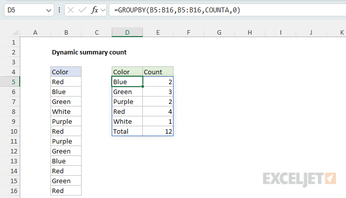
To create a summary count table that updates automatically, you can use the GROUPBY function with the COUNTA function. In the example shown, the formula in D5 is:

=GROUPBY(B5:B16,B5:B16,COUNTA,0)

The result is a table that spills into D5:E10, with each color in B5:B16 listed once, a count for each color, and a total row. GROUPBY is only available in Excel 365. In Excel 2021 and 2024, you can use UNIQUE and COUNTIF instead.

Generic formula

=GROUPBY(range,range,COUNTA,0)

Explanation

In this example, the goal is to build a simple summary count table with a formula. Once created, the summary table should automatically update to show new values and counts when data changes. This takes two steps: get a list of the unique colors in B5:B16, then count how many times each color appears. The article below walks through several options, including how to sort the table in descending order by count.

Why not a pivot table?
Summary count with GROUPBY
Sort by count
UNIQUE and COUNTIF
All-in-one formula with HSTACK
Which formula should you use?

Why not a pivot table?

A pivot table is one of the easiest ways to create a summary count, and it works in any version of Excel. If you use an Excel Table as the source data, the summary will stay in sync with the data. Also, the summary table can be easily sorted in a pivot table. However, a pivot table must be refreshed to see the latest data, and the solution is not a formula. Nevertheless, a pivot table is an excellent way to create a summary table.

Video: How to quickly create a pivot table

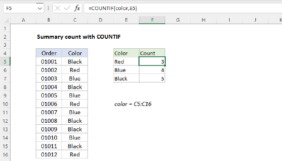
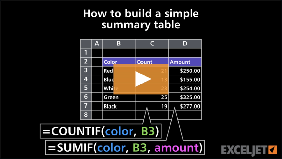
You can also build a summary table by hand: copy the values, use the Remove Duplicates command to get unique values, and then copy a COUNTIF formula down next to each value. This works fine, but the summary table will not update automatically if new values are added to the data. See Summary count with COUNTIF for this approach.

Video: How to build a simple summary table

Summary count with GROUPBY

The GROUPBY function is designed to group and summarize data, so it can extract the unique colors and count them in one step. In the worksheet shown, the formula in D5 is:

=GROUPBY(B5:B16,B5:B16,COUNTA,0)

Dynamic summary count with the GROUPBY function

Here are the arguments:

row_fields - B5:B16, because we want to group by color.
values - B5:B16 again, because the values to count are the colors themselves.
function - COUNTA, to count the values in each group.
field_headers - 0, because B5:B16 doesn't include a header. Be careful with this one: if you use 1, GROUPBY treats the first color as a header and leaves it out of the counts, so Red gets a count of 3 instead of 4.

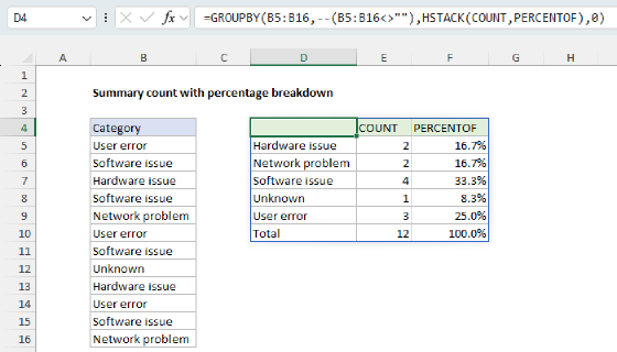
GROUPBY collects the five colors in B5:B16, counts the rows for each color, and returns the result as a table that spills into D5:E10. By default, GROUPBY sorts the colors from A to Z and adds a total row. The total of 12 is a quick check that every row was counted. To remove the total row, set total_depth to 0:

=GROUPBY(B5:B16,B5:B16,COUNTA,0,0)

Use COUNTA, not COUNT. COUNT counts only numbers, so with text values like these colors, GROUPBY returns a count of 0 for every color.

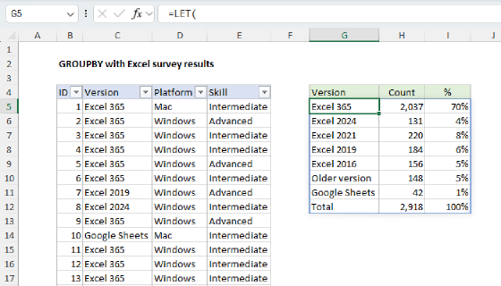
If you plan to add more data, put it in an Excel Table and use a structured reference like Table1[Color] in place of B5:B16, so new rows are included automatically. For other options, see GROUPBY with a dynamic range.

If the range includes empty cells (B5:B20, for example), GROUPBY adds a group labeled 0 that counts them. To leave them out, provide a test for empty cells as filter_array, and keep field_headers set to 0, since GROUPBY returns #VALUE! for this range when it is left out: =GROUPBY(B5:B20,B5:B20,COUNTA,0,,,B5:B20<>"").

Sort by count

GROUPBY sorts on the first column of the result by default, so the colors appear in A to Z order. To sort by count instead, with the largest count first, set sort_order to -2:

=GROUPBY(B5:B16,B5:B16,COUNTA,0,,-2)

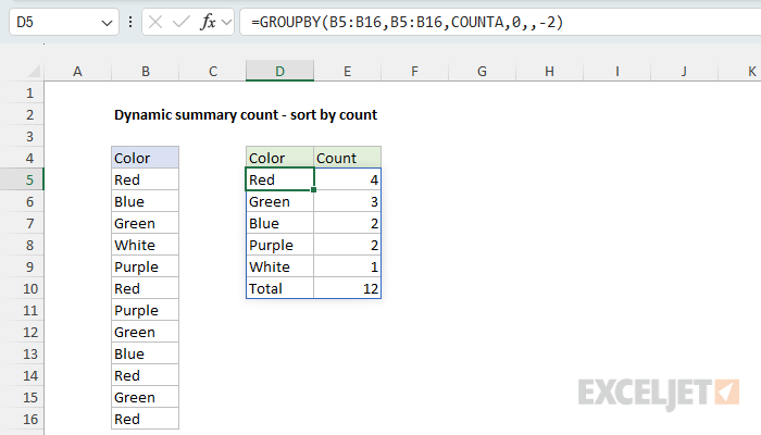
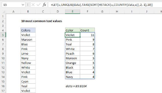
Dynamic summary count sorted by count with GROUPBY

The 2 refers to the second column of the result, which holds the counts, and the minus sign means descending order. The empty argument skips total_depth, so GROUPBY still adds a total row at the bottom. To list only the most common values, see 10 most common text values.

UNIQUE and COUNTIF

Another way to create a summary table is to use two formulas, one to collect unique values, and one to count the values. This approach works in Excel 2021 and later. It also lists the colors in the order they first appear in the data, which GROUPBY can't do, because GROUPBY always sorts its results. The formula in D5 is based on the UNIQUE function:

=UNIQUE(B5:B16) // get unique values

The formula in E5 uses the COUNTIF function:

=COUNTIF(B5:B16,D5#) // count unique values

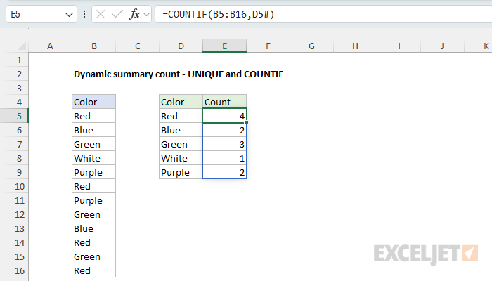
Dynamic summary count with UNIQUE and COUNTIF

Notice that inside COUNTIF, B5:B16 is provided as the range argument, and the spill reference D5# is used for criteria. Because D5# holds five colors, COUNTIF returns five counts, which spill into E5:E9. When source data changes, both formulas will stay in sync. In general this is a good, simple option. However, there are limitations. Because there are two separate formulas, we can't sort the results (in place) with the SORT function. And like the other *IFS functions, COUNTIF requires an actual range for the range argument, so it won't work when the data is an array returned by another formula. GROUPBY doesn't have this limitation.

All-in-one formula with HSTACK

To return the entire table with one formula, we can combine UNIQUE and COUNTIF with the HSTACK function. The formula in D5 is:

=LET(u,UNIQUE(B5:B16),HSTACK(u,COUNTIF(B5:B16,u)))

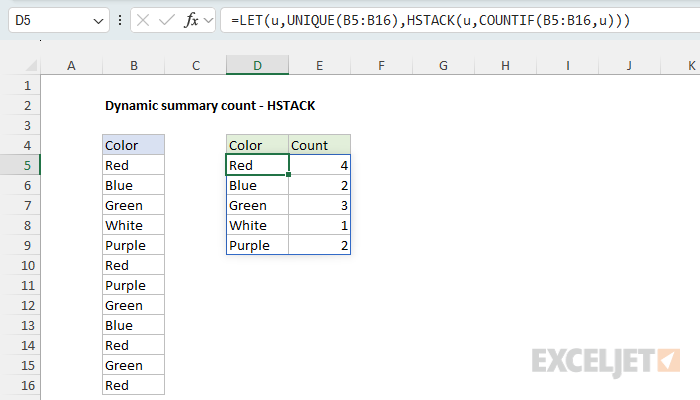
All-in-one formula for a dynamic summary count with HSTACK

The LET function defines a variable, u, to hold the unique values, so UNIQUE is called once only, and u is used twice. The count is essentially the COUNTIF formula explained above, except the criteria argument is u instead of a spill reference:

COUNTIF(B5:B16,u) // counts

HSTACK then combines the colors and the counts side by side into a single array, which displays as a two-column table in the worksheet.

Now that we have a formula that returns the entire table, we can sort the table in descending order by count. To do this, we wrap HSTACK in the SORT function, and specify 2 for sort_index and -1 for sort_order:

=LET(u,UNIQUE(B5:B16),SORT(HSTACK(u,COUNTIF(B5:B16,u)),2,-1))

This returns the same table as the GROUPBY formula in Sort by count, without the total row.

Video: Basic SORT function example

HSTACK is available in Excel 2024+ and Excel 365. In Excel 2021, use the CHOOSE function to combine the two arrays instead: =LET(u,UNIQUE(B5:B16),CHOOSE({1,2},u,COUNTIF(B5:B16,u))).

Which formula should you use?

In Excel 365, use GROUPBY. It's one short formula, it can sort by count, and it adds a total row.
To list the colors in the order they first appear, use UNIQUE and COUNTIF.
In Excel 2024, use UNIQUE, COUNTIF, and HSTACK in one formula, wrapped in SORT to sort by count.
In Excel 2021, use CHOOSE in place of HSTACK.
In any version of Excel, a pivot table is a good option, as long as you remember to refresh it.