CHOOSE Function

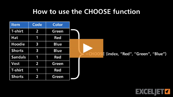
The CHOOSE function returns a value from a list using a position, or index. The first argument, index_num, is a number, and the arguments that follow are the values to choose from. When index_num is 1, CHOOSE returns the first value; when it is 2, CHOOSE returns the second value, and so on. CHOOSE is often used to convert a number into something more useful, like the name of a day or the quarter of a fiscal year.

What makes CHOOSE more interesting than it first appears is its flexibility: values can be text, numbers, cell references, or formulas. They can also be entire ranges, so CHOOSE can give a function like SUM or VLOOKUP a range selected with a number. And when index_num is an array of numbers, CHOOSE can return more than one value at a time, so it can combine columns into a new table. For many years, no other function could do these last two things, so CHOOSE turns up in many older formulas, where it can be hard to understand at first glance.

Other functions can handle some of these jobs more directly. The SWITCH function matches a value instead of a position, XLOOKUP can look up values in any direction, and HSTACK combines columns. The examples below cover each kind of value in turn, and mention when another function is a better choice.

Key features

• Converts a number into a value from a list you provide
• Selects by position: 1 returns the first value, 2 returns the second, and so on
• Values can be text, numbers, cell references, ranges, or formulas
• Short-circuit behavior: only calculates the value it returns
• Can return entire ranges to other functions like SUM, COUNTIF, and VLOOKUP
• Can return more than one value at a time when index_num is an array

Table of contents

• Basic examples
• Convert a number to a day name
• Get the fiscal quarter from a date
• Switch between scenarios
• Sum or look up in a selected table
• Combine columns with an array of index numbers
• CHOOSE versus other functions
• Notes

Basic examples

CHOOSE takes an index number followed by the values to choose from. The index number can be hard-coded, or it can come from a cell:

=CHOOSE(2,"red","blue","green") // returns "blue"
=CHOOSE(3,10,20,30) // returns 30
=CHOOSE(A1,"Low","Medium","High") // index number from A1

If the index number is less than 1 or greater than the number of values, CHOOSE returns a #VALUE! error:

=CHOOSE(4,"red","blue","green") // returns #VALUE!

The values can also be ranges. In that case, CHOOSE returns the selected range, which you can give to another function:

=CHOOSE(2,range1,range2) // returns range2
=SUM(CHOOSE(2,range1,range2)) // returns the sum of range2

One thing that confuses new users is that CHOOSE won't retrieve a value from inside a range. A range counts as one value, so the formula below returns #VALUE!, because the list has only one value to choose from:

=CHOOSE(2,A1:A3) // returns #VALUE!

To get the second value in a range, use the INDEX function or the CHOOSEROWS function instead:

=INDEX(A1:A3,2) // returns the value in A2
=CHOOSEROWS(A1:A3,2) // returns the value in A2

Convert a number to a day name

In the worksheet below, the goal is to convert the numbers 1 to 7 in column B into day names, where 1 is Monday and 7 is Sunday. The formula in D5, copied down, is:

=CHOOSE(B5,"Monday","Tuesday","Wednesday","Thursday","Friday","Saturday","Sunday")

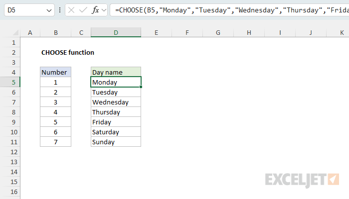
The number in column B is index_num, and the seven day names are the values. In D5, B5 contains 1, so CHOOSE returns "Monday", the first value. In D11, B11 contains 7, so CHOOSE returns "Sunday", the seventh value. Because the names are hard-coded into the formula, they can be anything you like, for example, custom abbreviations or names in another language.

In Excel 2021+, you can also give CHOOSE all the numbers at once. The formula below returns seven day names, which spill into D5:D11:

=CHOOSE(B5:B11,"Monday","Tuesday","Wednesday","Thursday","Friday","Saturday","Sunday")

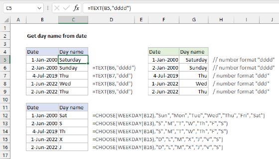
Typically, the goal is to get a day name from a date. The WEEKDAY function returns a number for the day of the week, and with a return_type of 2, Monday is 1 and Sunday is 7, which matches the list above. With a date in B5, this formula will return the correct day name:

=CHOOSE(WEEKDAY(B5,2),"Monday","Tuesday","Wednesday","Thursday","Friday","Saturday","Sunday")

The TEXT function is a simpler way to get a standard day name from a date: =TEXT(B5,"dddd") returns "Monday" for a date that falls on a Monday, and =TEXT(B5,"ddd") returns "Mon". However, CHOOSE is handy for custom names that TEXT can't create, like "Mo" and "Tu". See Get day name from date and Custom weekday abbreviation.

Get the fiscal quarter from a date

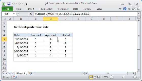
The values in CHOOSE don't have to be different from each other. In this example, the goal is to get the fiscal quarter for each date in column B, in a fiscal year that begins in April. The formula in D5, copied down, is:

=CHOOSE(MONTH(B5),4,4,4,1,1,1,2,2,2,3,3,3)

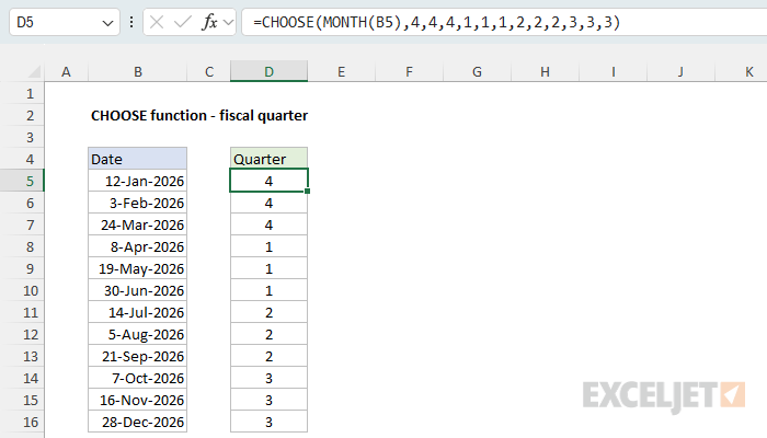
The MONTH function returns a number from 1 to 12, which becomes index_num, and CHOOSE returns one of 12 values, one for each month. January, February, and March fall in the fourth quarter of a fiscal year that begins in April, so the first three values are 4. April, May, and June fall in the first quarter, so the next three values are 1, and so on. In D8, the date is in April, so MONTH returns 4, and CHOOSE returns the fourth value, 1.

The nice thing about this formula is that the values read like the fiscal calendar, so it's easy to adapt to a different start month. For a fiscal year that begins in July, shift the values so that July is the first month of quarter 1:

=CHOOSE(MONTH(B5),3,3,3,4,4,4,1,1,1,2,2,2) // July start

To return a label like "Q1" instead of a number, concatenate "Q" to the result:

="Q"&CHOOSE(MONTH(B5),4,4,4,1,1,1,2,2,2,3,3,3)

For more details, see Get fiscal quarter from date.

Switch between scenarios

The values in CHOOSE can be cell references, which is one way financial models can switch between scenarios. In the worksheet below, columns C, D, and E hold Worst, Base, and Best values for four assumptions, and the scenario number in I5 picks one set of values. The formula in G5, copied down, is:

=CHOOSE($I$5,C5,D5,E5)

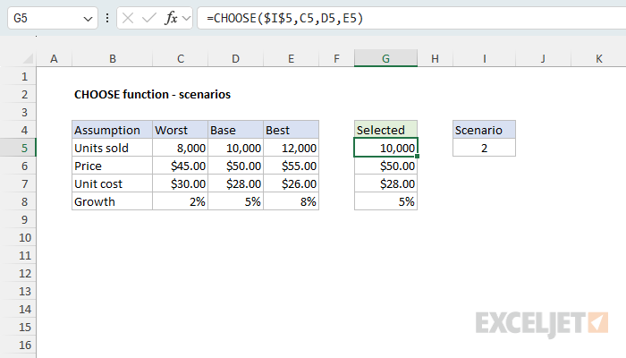
With 2 in I5, CHOOSE returns the second reference on each row, so column G shows the Base values. Change I5 to 3, and every row in column G switches to the Best values. The reference to I5 is absolute, so it doesn't change when the formula is copied down, while C5, D5, and E5 are relative and move down one row at a time. In a model, the calculations refer only to column G, so the one number in I5 drives every result.

Because each scenario's four values sit together in one range, you could also select all of them in one step. In Excel 2021+, this single formula in G5 returns the four values for the selected scenario, which spill into G5:G8:

=CHOOSE(I5,C5:C8,D5:D8,E5:E8)

This is a good example of the flexibility CHOOSE offers: it can return ranges in addition to single values.

To pick a scenario by name instead of by number, use the XMATCH function to convert the name into a position. With "Best" in I5, this formula returns 12,000 in G5:

=CHOOSE(XMATCH($I$5,{"Worst","Base","Best"}),C5,D5,E5)

When the scenarios sit side by side under headers, as they do here, XLOOKUP can do the same job with a scenario name in I5: =XLOOKUP($I$5,$C$4:$E$4,C5:E5). CHOOSE is more flexible, because its values can be anywhere: on other sheets, in separate blocks, or calculated by formulas.

Sum or look up in a selected table

When a value in CHOOSE is a range, CHOOSE returns the range itself, not just its values. This means you can give the result to a function that expects a range. In the worksheet below, there are three Excel Tables named East, West, and North, and the table number in K5 selects one of them. The formula in K8 sums the sales in the selected table:

=SUM(CHOOSE(K5,East[Sales],West[Sales],North[Sales]))

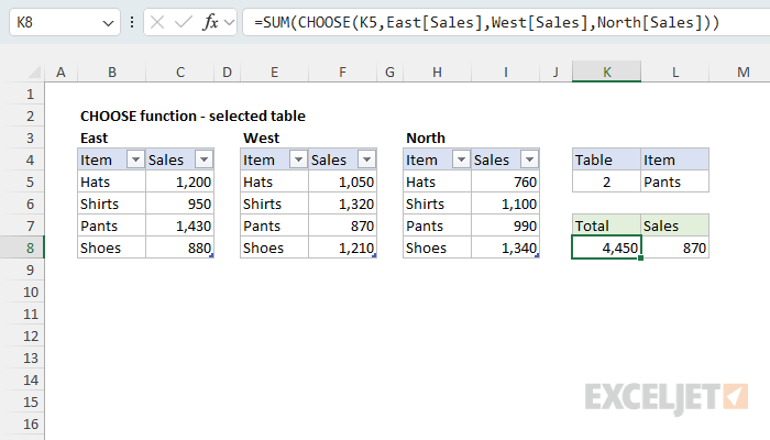
With 2 in K5, CHOOSE returns West[Sales], and SUM returns 4,450, the total for the West table. The formula in L8 uses the same idea to look up the item in L5:

=VLOOKUP(L5,CHOOSE(K5,East,West,North),2,0)

Here, CHOOSE returns the entire West table, which VLOOKUP uses as table_array. VLOOKUP finds "Pants" in the first column and returns 870 from the second column. Change K5 to 1 or 3, and both formulas switch to the East or North table.

The fact that CHOOSE returns a range can be handy in other ways. Some functions, including SUMIFS and COUNTIF, require a range for certain arguments and won't accept an array (see SUMIF quirks). Because CHOOSE returns a range, it works with these functions too. For example, this formula counts sales over 1,000 in the selected table and returns 3:

=COUNTIF(CHOOSE(K5,East[Sales],West[Sales],North[Sales]),">1000")

For a similar example with INDEX and MATCH, see INDEX with variable array.

CHOOSE works well for a handful of tables. But typically, a better approach is to keep all data in one table with a column for the region, then use the region as criteria in a function like SUMIFS or FILTER. If the data is already split across tables, the VSTACK function can combine them.

Combine columns with an array of index numbers

For such an old function, CHOOSE has a few novel tricks that power users have exploited over the years. One of these is the ability to combine columns using an array of index numbers. You'll see this in older lookup formulas like this one, which looks up a value to the left:

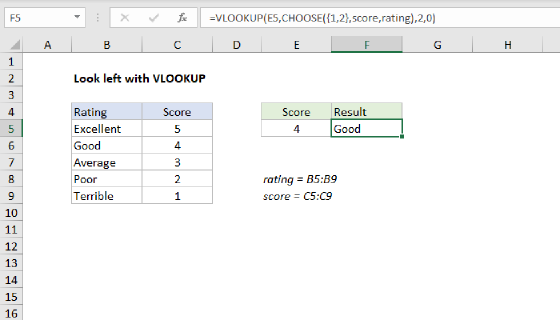
=VLOOKUP(I5,CHOOSE({1,2},D5:D12,B5:B12),2,0)

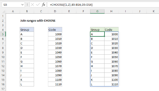
This is a CHOOSE pattern that confuses many people. How does it work? The key is that index_num is an array constant, {1,2}, so CHOOSE runs once for each number and returns both results side by side. To see this, it helps to look at CHOOSE on its own. In the worksheet below, the formula in F5 is:

=CHOOSE({1,2},B5:B12,D5:D12)

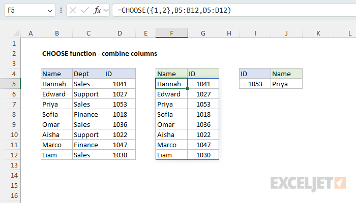
The 1 in {1,2} returns the first range, B5:B12 (the names), and the 2 returns the second range, D5:D12 (the IDs). Because {1,2} is a horizontal array (a comma separates columns in an array constant), the two ranges land in two columns, and the result spills into F5:G12. The result is a new two-column table without the Dept column. The power user trick is that you can reverse the numbers to reorder the columns:

=CHOOSE({2,1},B5:B12,D5:D12) // IDs first, then names

Now back to the lookup formula in J5. VLOOKUP can only look to the right of the first column in a table, but the goal is to look up an ID and return a name, which sits to the left of the ID. To solve this problem, the formula uses the trick above: CHOOSE builds a table in memory with the IDs first:

CHOOSE({1,2},D5:D12,B5:B12) // IDs, then names

VLOOKUP then matches 1053 in the first column of this table and returns "Priya" from the second column. For a full explanation, see Left lookup with VLOOKUP and Combine ranges with CHOOSE.

The trick above has some limitations and quirks you should be aware of:

• With a semicolon, {1;2}, the array is vertical, and CHOOSE does not stack the ranges. Instead, it returns one column: the first row of the first range, the second row of the second range, and #N/A errors after that. To stack ranges, use the VSTACK function.
• When a range has more than one column, CHOOSE uses only the first column.
• When the ranges have different numbers of rows, the shorter one is padded with #N/A errors.
• A single value, like "East", repeats down every row. (HSTACK pads a single value with #N/A errors instead.)
• Text longer than 255 characters returns #VALUE!, so a left lookup that returns long descriptions can fail, where XLOOKUP returns the full text.

The same idea works with separate cells: =CHOOSE({1,2,3},A1,C5,E9) returns the three values as one horizontal array, which you can give to another function.

CHOOSE versus other functions

CHOOSE is an older function in Excel. If you need to select a value with a numeric index and the list of values is not too long, there is no reason not to use it. However, many newer functions have similar and overlapping abilities:

• The SWITCH function matches a value instead of a position, so it works with text and codes that aren't numbered 1, 2, 3, and it can return a default when nothing matches. See SWITCH versus CHOOSE.
• The XLOOKUP function looks to the left as well as the right, so it doesn't need CHOOSE to rearrange columns for VLOOKUP: =XLOOKUP(I5,D5:D12,B5:B12) returns the same result as the formula in J5 above.
• The HSTACK function combines ranges side by side, and the VSTACK function stacks them vertically.
• The CHOOSECOLS function selects and reorders columns in one range by number: =CHOOSECOLS(B5:D12,1,3) returns the same table as the formula in F5 above. The CHOOSEROWS function does the same for rows.

SWITCH is available in Excel 2019+, XLOOKUP in Excel 2021+, and HSTACK, VSTACK, CHOOSECOLS, and CHOOSEROWS in Excel 2024+. All of them are available in Excel 365. CHOOSE is still the answer in Excel 2021, which has XLOOKUP but not HSTACK or CHOOSECOLS. It's also worth understanding in any version, because it turns up in so many older formulas.

Notes

• CHOOSE returns #VALUE! when index_num is less than 1 or greater than the number of values.
• When index_num is a decimal, CHOOSE truncates it: 2.9 fetches the second value, and 0.5 returns #VALUE!.
• A number entered as text works as index_num, so "2" returns the second value. TRUE returns the first value, and FALSE returns #VALUE!.
• A range counts as one value. =CHOOSE(2,A1:A3) returns #VALUE!, and =CHOOSE(1,A1:A3) returns the whole range, which spills in Excel 2021+.
• An empty value returns zero: =CHOOSE(2,"a",,"c") returns 0. So does a reference to an empty cell.
• CHOOSE calculates only the value it returns, so an error or a slow calculation in another value has no effect.
• In a recursive LAMBDA formula, CHOOSE stops the recursion just like IF does, where IFS and SWITCH return #NUM!.
• When index_num is an array, text values longer than 255 characters return #VALUE!. With a single index number, CHOOSE returns the full text.
• CHOOSE can handle up to 254 values.