Summary
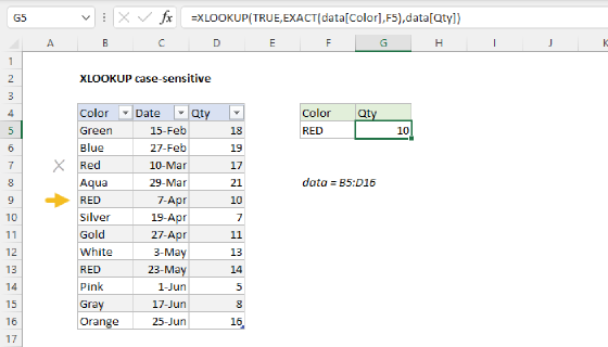
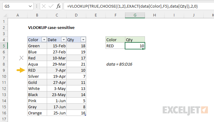
To create a case-sensitive lookup with the VLOOKUP function, you can use the EXACT function. In the example shown, the formula in G5 is:
=VLOOKUP(TRUE,CHOOSE({1,2},EXACT(data[Color],F5),data[Qty]),2,0)
where "data" is an Excel Table in the range B5:D16. In this configuration, VLOOKUP matches the text "RED" in row 5 of the table and returns 10 from the Qty column in the same row. This is an array formula and must be entered with control + shift + enter, except in Excel 365 or Excel 2021.
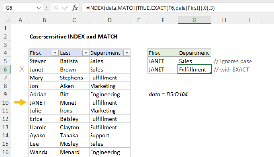
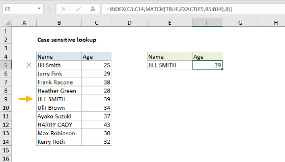
Note: With XLOOKUP, or INDEX and MATCH, the approach is the same but the formulas are more straightforward: XLOOKUP example, INDEX and MATCH example.
Generic formula
=VLOOKUP(TRUE,CHOOSE({1,2},EXACT(range1,A1),range2),2,0)
Explanation
In this example, the goal is to perform a case-sensitive lookup on Color with VLOOKUP. In other words, a lookup value of "RED" must return a different result from a lookup value of "Red". This presents several challenges. First, Excel is not case-sensitive by default, and there is no built-in setting to make VLOOKUP case-sensitive. For example, if we try a standard VLOOKUP formula in exact match mode, we get the wrong result:
=VLOOKUP("RED",data,3,0) // returns 17
VLOOKUP matches "Red" in row 3, and returns 17. The correct result is 10.
The second challenge is the table itself. Unlike XLOOKUP or INDEX and MATCH, VLOOKUP requires the entire table to be provided in the table_array argument. Normally, this is not a problem. However, to enable a case-sensitive VLOOKUP, we can't use the existing table as-is, and this means we need to take special steps to assemble a table that will work for this problem.
The overall process looks like this:
- Use the EXACT function to check the Color column for the lookup value.
- Join the results from EXACT to the Qty column with the CHOOSE function.
- Provide the resulting array to VLOOKUP as the table_array argument.
- Configure VLOOKUP to look for TRUE in the new table.
The result is a case-sensitive lookup with VLOOKUP. Read on for a complete explanation.
Background reading
This article assumes you are familiar with the VLOOKUP function and Excel Tables. If not, see:
- Excel Tables - introduction and overview
- VLOOKUP function - overview with examples
- EXACT function - overview
EXACT function
The EXACT function is designed to perform a case-sensitive comparison of two text values. If the two values match exactly, EXACT returns TRUE. If not, EXACT returns FALSE. The twist in this case is that we need to check every value in the Color column against the value in F5. Fortunately, the EXACT function will do this.
Working from the inside out, we set up the EXACT function like this:
=EXACT(data[Color],F5)
Since there are 12 values in the Color column, the EXACT function will return a vertical array with 12 TRUE and FALSE results like this:
{FALSE;FALSE;FALSE;FALSE;TRUE;FALSE;FALSE;FALSE;FALSE;FALSE;FALSE;FALSE}
Notice the position of TRUE (5) corresponds to row 5 in the table, where Color is "RED". EXACT returns FALSE for every other value, including "Red" in row 3. This gives us an array we can use in the next step.
CHOOSE function
We now have an array of TRUE and FALSE values that will function as a key to which row(s) in the table match "RED". The problem is that the array is not actually part of the table, and VLOOKUP needs an entire table as the table_array argument. In addition, the first column in the table must contain lookup values. What we need is a new table, that combines the result from EXACT with the values in the Qty column.
Enter the CHOOSE function. Normally, the CHOOSE function is used to select a value by numeric position. For example, to get the second value from a list of three values, you could use CHOOSE like this:
=CHOOSE(2,value1,value2,value3) // returns value2
CHOOSE is flexible when it comes to values, which can be any mix of constants, cell references, arrays, or ranges. In this case, we give CHOOSE the array created by the EXACT function as value1 and the Qty column in the table as value2. Then, for index_num, we provide the array constant {1,2} like this:
=CHOOSE({1,2},EXACT(data[Color],F5),data[Qty])
The array constant is the tricky part. By using the array {1,2} we are requesting value1 and value2 at the same time. As a result, the array from EXACT and data[Qty] are "glued" together and returned as a single array. This array only exists in memory, but it looks like this:
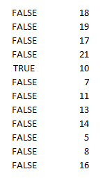
As you can see, the array has 2-columns. We now have a table we can use in VLOOKUP.
Note: whenever you see =CHOOSE({1,2} you should think "2 things are being joined together".
VLOOKUP function
Next, we need to connect the code above to the VLOOKUP function. We know the first column in the array we created contains TRUE or FALSE values, so we start with a lookup value of TRUE:
=VLOOKUP(TRUE,
This may seem strange, but remember that the original color values are gone (replaced by TRUE and FALSE) and so we need to look for TRUE and not "RED". Next, for the table_array argument, we add the code that creates our custom table:
=VLOOKUP(TRUE,CHOOSE({1,2},EXACT(data[Color],F5),data[Qty])
The array created by CHOOSE is returned directly to the VLOOKUP function as the table_array argument. Because the values we want to retrieve are in the second column, we set col_index_num to 2. Then we set the range_lookup argument to zero or FALSE, to enable an exact match. The final formula in G5 is:
=VLOOKUP(TRUE,CHOOSE({1,2},EXACT(data[Color],F5),data[Qty]),2,0)
VLOOKUP matches the text "RED" in row 5 of the table and returns 10 as a final result.
Note: This is an array formula and must be entered with control + shift + enter, except in Excel 365 or Excel 2021.