Summary
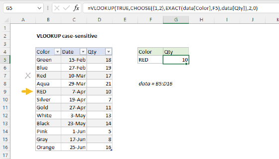
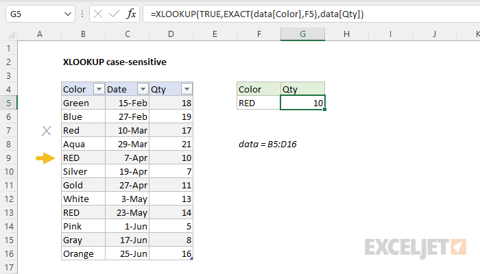
To create a case-sensitive lookup with the XLOOKUP function, you can use the EXACT function. In the example shown, the formula in G5 is:
=XLOOKUP(TRUE,EXACT(data[Color],F5),data[Qty])
where "data" is an Excel Table in the range B5:D16. The result is that XLOOKUP matches the text "RED" in row 5 of the table and returns 10 from the Qty column in the same row.
Generic formula
=XLOOKUP(TRUE,EXACT(range1,A1),range2)
Explanation
In this example, the goal is to perform a case-sensitive lookup on the color in the "Color" column. In other words, a lookup value of "RED" must return a different result from a lookup value of "Red". By default, Excel is not case-sensitive and this applies to standard lookup formulas like VLOOKUP, XLOOKUP, and INDEX and MATCH. These formulas will simply return the first match, ignoring case. For example, if we use a standard XLOOKUP formula like this:
=XLOOKUP("RED",data[Color],data[Qty]) // returns 17
XLOOKUP will match "Red" in row 3 of the table and return 17, even though the lookup value is "RED" in uppercase.
We need a way to get Excel to compare case. The EXACT function is perfect for this job, but the way we use it is a little different. Instead of comparing one text value to another, we compare one text value to many values. In a nutshell, we use the EXACT function to generate an array of TRUE and FALSE values, then use the XLOOKUP function to locate the first TRUE in the array.
Like many advanced formulas in Excel, this approach requires you to imagine what the formula is doing, even though the process is largely invisible. There is no shortcut to mastering these ideas, you just have to practice :)
Background reading
This article assumes you are familiar with the XLOOKUP function and Excel Tables. If not, see:
- Excel Tables - introduction and overview
- Basic XLOOKUP example - 3-minute video
EXACT function
Working from the inside out, to give XLOOKUP the ability to match case, we use the EXACT function like this:
EXACT(data[Color],F5)
Since there are 12 values in the Color column, the EXACT function will return an array with 12 TRUE and FALSE results like this:
{FALSE;FALSE;FALSE;FALSE;TRUE;FALSE;FALSE;FALSE;TRUE;FALSE;FALSE;FALSE}
Notice the position of the first TRUE (5) corresponds to row 5 in the table, where Color is "RED". EXACT returns TRUE again for "RED" in row 9 of the table. Every other result is FALSE, including "Red" in row 3.
XLOOKUP with EXACT
As explained above, the EXACT function creates an array of TRUE and FALSE values, one for each value in the Color column. This array is returned directly to the XLOOKUP function as the lookup_array argument. Now we need to give XLOOKUP an appropriate lookup_value. Instead of looking for "RED" (the original lookup value), we provide the value TRUE. This may seem a bit strange, but remember that when the EXACT function runs, it returns an array of TRUE/FALSE values. The original values are gone and thus we need to look for TRUE and not "RED".
Finally, we need to provide a return_array. This is the column that contains the values we want as a result. In this example, return_array is the last column in the table, data[Qty]. The final formula in cell G5 looks like this:
=XLOOKUP(TRUE,EXACT(data[Color],F5),data[Qty]) // returns 10
In summary, the EXACT function compares the value in F5 with every value in data[Color], generating an array of TRUE and FALSE values. This array is returned to XLOOKUP as the lookup_array. XLOOKUP locates the TRUE at position 5 in the array and returns the value at row 5 in the Qty column, 10 as a final result.
Notice that XLOOKUP matches on the first TRUE and not the second and last TRUE. This is standard behavior for Excel's lookup functions when there is more than one match.
Alternate syntax
You may sometimes see an alternate syntax like this:
=XLOOKUP(1,--EXACT(data[Color],F5),data[Qty]) // returns 10
The behavior of this formula is the same. However, in this version, we convert the TRUE and FALSE values returned by EXACT to 1s and 0s with the double negative:
--EXACT(data[Color],F5) // convert to 1s and 0s
This yields an array like this:
{0;0;0;0;1;0;0;0;1;0;0;0}
The positions of the 1s in this array correspond to the rows where the color is "RED". This array is returned directly to the XLOOKUP function as the lookup array argument. We can now rewrite the formula like this:
=XLOOKUP(1,{0;0;0;0;1;0;0;0;1;0;0;0},data[Qty])
With a lookup value of 1, XLOOKUP finds the 1 in the 5th position and again returns the value at row 5 in the Quantity column: 10.
This use of 1s and 0s is common in formulas that use Boolean logic because Excel automatically coerces TRUE and FALSE values to 1s and 0s during any math operation. See below for an example.
Extending the logic
The structure of the logic can be easily extended. For example, to narrow the match to "RED" in May, you can use a formula like this:
=XLOOKUP(1,EXACT(data[Color],F5)*(MONTH(data[Date])=5),data[Qty])
Here, because each of the two expressions returns an array of TRUE FALSE values, and because these arrays are multiplied together, the math operation coerces the TRUE and FALSE values to 1s and 0s. It is not necessary to use the double-negative. The lookup value remains 1, as in the formula above. Once this operation is complete, the formula looks like this:
=XLOOKUP(1,{0;0;0;0;0;0;0;0;1;0;0;0},data[Qty])
XLOOKUP locates the 1 in the 9th position and returns 14 as a final result
First and last match
If there is more than one match in lookup_array, XLOOKUP will return the first match by default. To force XLOOKUP to return the last match, set the search mode argument for XLOOKUP to -1:
=XLOOKUP(1,--EXACT(data[Color],F5),data[Qty],,,-1) // last match
This version of the formula will return 14 as a final result.
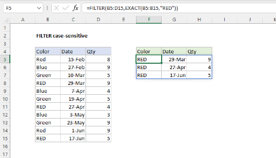
If you need to return multiple results for multiple matches, see the FILTER function.